Readings for Unit 5

Licensing Information

The readings for 6.s090 are licensed under a Creative Commons Attribution-NonCommercial-ShareAlike 4.0 International License. You are free to make and share verbatim copies (or modified versions) under the terms of that license.

Portions of these readings were modified or copied verbatim from the very nice book Think Python 2e by Allen Downey.

PDF of these readings also available to download: 6s090_reading5.pdf

Table of Contents

1) Introduction

As we have learned throughout the course, functions allow us to abstract away the details of a particular computation so that it can be computed multiple times on different inputs. This week's readings will, first, revisit the details of how Python interprets functions. In particular, we'll focus on the issue of scoping (deciding how and where Python looks up variable names). Then, we'll discuss the "first-class" nature of Python functions and other useful features. We'll also discuss some new ways to test our code and how to use external packages.

2) More Functions

To begin, we will step through a complex function example with an environment diagram. This builds upon the things we learned in unit 3's reading, so you may wish to review those now.

2.1) Environment Diagram Review

First, let's walk through the following piece of (admittedly silly) code:

def f(x):
    x = x + y
    print(x)
    return x

def g(y):
    y = 17
    return f(x+2)

x = 3
y = 4
z = f(6)

a = g(y)

print(z)
print(a)
print(x)
print(y)

Try to use an environment diagram to predict what values will be printed to the screen as this program runs. You can step through our explanation of how this code runs using the buttons below:

<< First Step  < Previous Step  Next Step > Last Step >>

Explanations go here.

2.2) A Mystery Program

If you find these diagrams tedious, we get it... In the end, there's a reason we want computers to be the one doing this, after all; they're much better at these operations than we are, and much faster! So, in the short term, this is tedious. But the long-term benefits are really great! This kind of practice is helpful in building up a mental model of Python's behavior, which is important so that when you encounter unexpected behavior, you can come back to the model. With practice, this kind of thinking will become second nature, and you won't have to draw these diagrams out in such detail.

To motivate why environment diagrams might be useful, let's look at another example of a mystery Python program:

functions = []
for i in range(5):
    def func(x):
        return x + i
    functions.append(func)

for f in functions:
    print(f(12))

Without running this code, take a few moments to predict what is going to happen when it is run. Which of the following do you think is going to happen?

It prints 12, then 13, then \ldots, then 16

It prints 13, then 14, then \ldots, then 17

It prints 16, then 15, then \ldots, then 12

It prints 17, then 16, then \ldots, then 13

A Python error occurs

Something else

Loading...

Now, only once you have made an educated guess above, type this code into your favorite text editor or IDE and run it. Does the result match your expectation?

2.3) Functions Are First-Class Objects

We now shift gears to learn about a powerful feature of Python: that it treats functions as first-class objects, which means that functions in Python can be manipulated in many of the same ways that other objects can be (specifically, they can be passed as arguments to other functions, defined inside of other functions, returned from other functions, and assigned to variables). In this section, we will explore how we can make use of this feature in our programs.

2.3.1) Function Names are Variable Names

In a previous unit, we encountered the round function that can round a number to a given number of decimal places. For example:

x = int(4.999)  # int always rounds down
y = round(4.5)  # round will round up or down
print(x, y) # 4 5

But what would happen if we took away the parentheses and didn't call the function?

r = round
print(r) # <built-in function round>
print(r(2.4))  # 2

It turns out that we can assign multiple variable names to the same function object in memory. The code above makes r and round aliases to the same built-in function object. This allows us to call r just like round. This is also the idea behind passing functions in as arguments to function calls, as we will see in the next section.

2.3.2) Functions as Arguments

Imagine that you wanted to make plots of several different functions. To do that, you would need to figure out which "y" values correspond to each of a number of "x" values. The following code computes these "y" values for different functions:

import math

def sine_response(lo, hi, step):
    y_vals = []
    x = lo
    while x <= hi:
        y_vals.append(math.sin(x))
        x += step
    return y_vals

def cosine_response(lo, hi, step):
    y_vals = []
    x = lo
    while x <= hi:
        y_vals.append(math.cos(x))
        x += step
    return y_vals

def double_response(lo, hi, step):
    y_vals = []
    x = lo
    while x <= hi:
        y_vals.append(x * 2)
        x += step
    return y_vals

def square_response(lo, hi, step):
    y_vals = []
    x = lo
    while x <= hi:
        y_vals.append(x**2)
        x += step
    return y_vals

if __name__ == "__main__":
    print(sine_response(0, math.pi/2, math.pi/8))
    # [0.0, 0.3826834323650898, 0.7071067811865476, 0.9238795325112867, 1.0]
    print(cosine_response(0, math.pi/2, math.pi/8))
    # [1.0, 0.9238795325112867, 0.7071067811865476, 0.38268343236508984, 6.123233995736766e-17]
    print(double_response(0, 2, .5))
    # [0, 1.0, 2.0, 3.0, 4.0]
    print(square_response(0, 2, .5))
    # [0, 0.25, 1.0, 2.25, 4.0]

Now imagine that instead of just wanting a list of y-values, you wanted these functions to return two lists, one to represent the x-values, and one to represent the y-values. Making this change or changing anything at all about this program would be a pain because you would have to manually change each of the above functions.

One way to make changing a program easier is to write it in a way that avoids repetition. After all, sine_response, cosine_response, double_response, and square_response are almost exactly the same, except for how the y-values get calculated. It would be nice if instead of four functions we could write a single function that could use different equations.

It turns out, we can cut down on a lot of this repetition by creating a more general function called response, which takes in a function f in addition to the other inputs.

def response(f, lo, hi, step):
    y_vals = []
    x = lo
    while x <= hi:
        y_vals.append(f(x))
        x += step
    return y_vals

Notice that, inside of the definition of response, we call f, the function that was passed in as an argument. Using response, we could compute the same y-values as the sine_response function as follows:

# These two compute the same response!
y1 = sine_response(0, math.pi/2, math.pi/8)
print(y1) # [0.0, 0.3826834323650898, 0.7071067811865476, 0.9238795325112867, 1.0]
y2 = response(math.sin, 0, math.pi/2, math.pi/8)
print(y2) # [0.0, 0.3826834323650898, 0.7071067811865476, 0.9238795325112867, 1.0]

When we pass in math.sin as an argument, we do not put parentheses after it. This is because we want to refer to the function itself (which is called math.sin), and not to any particular output of the function (which we'd get by calling it, such as in math.sin(7)).

y1 = double_response(0, 2, 0.5)
print(y1)
y2 = response(2 * x, 0, 2, 0.5)
print(y2)

y1 = double_response(0, 2, 0.5)
print(y1)  # [0, 1.0, 2.0, 3.0, 4.0]
y2 = response(2 * x, 0, 2, 0.5)
print(y2)  # NameError: name 'x' is not defined

x = 5
y2 = response(2 * x, 0, 2, 0.5)  # TypeError: 'int' object is not callable
print(y2)  # The program does not execute this line because of the error

x = 5
f = x * 2
print(f(x))  # equivalent to print(10(x))
# TypeError: 'int' object is not callable

We can recreate the behavior of double_response with response by creating a function to double individual values:

def double(x):
    return 2 * x

y1 = double_response(0, 2, 0.5)
print(y1)  # [0, 0.5, 1.0, 1.5, 2.0]
y2 = response(double, 0, 2, 0.5)   # note double is passed in without using ()!
print(y2)  # [0, 0.5, 1.0, 1.5, 2.0]

import math

def response(f, lo, hi, step):
    y_vals = []
    x = lo
    while x <= hi:
        y_vals.append(f(x))
        x += step
    return y_vals

def double(x):
    return 2 * x

def square(x):
    return x ** 2

if __name__ == "__main__":
    print(response(math.sin, 0, math.pi/2, math.pi/8))
    # [0.0, 0.3826834323650898, 0.7071067811865476, 0.9238795325112867, 1.0]
    print(response(math.cos, 0, math.pi/2, math.pi/8))
    # [1.0, 0.9238795325112867, 0.7071067811865476, 0.38268343236508984, 6.123233995736766e-17]
    print(response(double, 0, 2, .5))
    # [0, 1.0, 2.0, 3.0, 4.0]
    print(response(square, 0, 2, .5))
    # [0, 0.25, 1.0, 2.25, 4.0]

2.4) Understanding the Mystery Program

Earlier, we looked at the following piece of code as an example of code that is difficult to understand:

functions = []
for i in range(5):
    def func(x):
        return x + i
    functions.append(func)

for f in functions:
    print(f(12))

It is somewhat surprising that, despite the looping structure here, when we run this code, we see five 16's printed to the screen! Despite the surprising nature of this example, though, we now have all of the tools we need in order to make sense of this example and to understand why it behaves the way it does. We'll walk through an environment diagram to explain this behavior, and you're strongly encouraged to follow along (and to reach out for help if any of the steps are unclear!).

We'll start by drawing the diagram just for the first segment of the code (lines 1-5, where we are building up the functions list). Again, we encourage you to try to stay one step ahead of the drawings below (that is, try to draw out how things will change during each step, then click ahead and compare your work against our diagram).

<< First Step  < Previous Step  Next Step > Last Step >>

Explanations go here.

2.5) Default and Keyword Arguments

For functions we've seen so far, we indicate the arguments by positions. For example, with this function:

def percent(num, total):
    if not total:
        # avoid divide by 0 errors
        return f'0?'
    else:
        return f'{(num / total):.1%}'

print(percent(7, 0))  # 0?
print(percent(7, 11)) # 63.6%

When we call percent(7, 11), python knows that num should be 7 and total should be 11 because that's the order we defined the arguments to come in.

However, there is another way to pass in arguments, using the name instead of the position. For example, we write the argument name, an equal sign, and the value we want it to take on.

print(percent(total=11, num=7)) # this would still print '63.6%'

Finally, there's a way to specify a function to have optional arguments. We signify these arguments with a variable name as usual, but we also add an equal sign and a default value. For example, if we wanted our function to have the option of adding the fraction in addition to the percent, we could add the optional argument verbose.

def percent(num, total, verbose=False):
    extra = ''
    if verbose:
        extra = f' ({num}/{total})'

    if not total:
        # avoid divide by 0 errors
        return f'0?{extra}'
    else:
        return f'{(num / total):.1%}{extra}'

Note that we can still call percent like we did before. If we don't specify a value for verbose it will be False by default as we indicated in the function definition.

print(percent(7, 11))  # prints 63.6%

But we can also specify a value for verbose. For example:

print(percent(7, 11, verbose=False)) # 63.6%
print(percent(7, 11, verbose=True))  # 63.6% (7/11)

It's common practice to use keyword specification for optional arguments because if there are multiple default arguments, it's not immediately clear which ones are being set. For example, we can add another default argument to change the number of digits to round the percentage to as follows:

def percent(num, total, n=1, verbose=False):
    extra = ''
    if verbose:
        extra = f' ({num}/{total})'

    if not total:
        # avoid divide by 0 errors
        return f'0?{extra}'
    else:
        return f'{(num / total):.{n}%}{extra}'


print(percent(7, 11)) # 63.6%
print(percent(7, 11, n=5)) # 63.63636%
print(percent(7, 11, n=0, verbose=True)) # 64% (7/11)

It turns out that default arguments are what allow some of the built-in functions like round to take in different numbers of arguments, as we saw in unit 3's readings.

3) Assert statements

So far, we have debugged and tested our programs mainly with print statements. However, Python comes with additional tools to help us test whether our code actually does what we intend.

Assert statements check a conditional statement. If the statement evaluates to True, the program continues as normal, but if it evaluates to False an AssertionError will be raised and stop the program.

>>> assert 5 > 4 # evaluates to True, does nothing
>>> assert 5 < 4
...
AssertionError

For example, we could test the add_s function below with assert statements with the following code:

def add_s(words):
    """
    Given a list of words, output a new list of words with s added to
    the end without modifying the input.
    """
    new_words = []
    for word in words:
        new_words.append(word + "s")
    return new_words

if __name__ == '__main__':
    assert add_s(['can', 'add', 's']) == ['cans', 'adds', 'ss']
    assert add_s(['']) == ['s']
    assert add_s([]) == []
    print("done testing")

While this program only prints done testing, it also silently checks that the output matches what we expect, saving us from the hassle of manually checking whether the printed output is correct or not.

We can optionally add a string at the end of the assert statement to provide a more descriptive error message:

x = 5
y = 4
assert y > x, f'{y=} is not greater than {x=}!'
# AssertionError: y=4 is not greater than x=5!

We can also use assert statements within functions to check that the input is valid. For example:

def square(num):
    assert type(num) == float or type(num) == int, f"Expected float or int, got {num} which is a {type(num)}."
    return num ** 2

print(square(5))
print(square("uh oh"))

Outputs:

25
...
AssertionError: Expected float or int, got uh oh which is of <class 'str'>.

4) import statements

So far, we have explored a number of features that are built-in to Python. But sometimes, we want to split a large program into multiple smaller files or use a package that someone else wrote without having to manually copy and paste all of their code into our program. import statements are useful for exactly these kinds of situations.

For example, earlier we saw import math as part of our response program. This finds and imports a module called math, which becomes a variable in our program. To use the constant pi or the sin function which are defined within math, we need to use dot notation as follows:

import math
print(math)     # <module 'math' (built-in)>
print(math.pi)  # 3.141592653589793
print(math.sin) # <built-in function sin>
print(pi)       # NameError: name 'pi' is not defined

It turns out, the math module contains quite a number of things, which we can see using the dir command.

import math
print(dir(math))
"""
['__doc__', '__loader__', '__name__', '__package__', '__spec__', 'acos', 'acosh', 'asin', 'asinh', 'atan', 'atan2', 'atanh', 'cbrt', 'ceil', 'comb', 'copysign', 'cos', 'cosh', 'degrees', 'dist', 'e', 'erf', 'erfc', 'exp', 'exp2', 'expm1', 'fabs', 'factorial', 'floor', 'fma', 'fmod', 'frexp', 'fsum', 'gamma', 'gcd', 'hypot', 'inf', 'isclose', 'isfinite', 'isinf', 'isnan', 'isqrt', 'lcm', 'ldexp', 'lgamma', 'log', 'log10', 'log1p', 'log2', 'modf', 'nan', 'nextafter', 'perm', 'pi', 'pow', 'prod', 'radians', 'remainder', 'sin', 'sinh', 'sqrt', 'sumprod', 'tan', 'tanh', 'tau', 'trunc', 'ulp']
"""

We can avoid using math. and selectively import only what we want to use with from PACKAGE import THING1, THING2, ... as follows:

from math import pi, sin
print(pi)    # 3.141592653589793
print(sin)   # <built-in function sin>
print(math)  # NameError: name 'math' is not defined. Did you forget to import 'math'?

Or we can avoid using math. and import everything using from PACKAGE import * as follows:

from math import *
print(pi)    # 3.141592653589793
print(sqrt)  # <built-in function sqrt>
print(math)  # NameError: name 'math' is not defined. Did you forget to import 'math'?

Programmers like to use short abbreviations, especially for commonly imported modules like pandas (pd), numpy (np), and matplotlib.pyplot (plt). We can import a package and give it a different name with import LONG_PACKAGE as PACKAGE:

import pandas as pd
print(pd) # <module 'pandas' from SOME/LONG/FILE/PATH/__init__.py>
print(pandas) # NameError: name 'pandas' is not defined

This is essentially the same as importing a package and then re-naming it without needing to use two different variable names:

import pandas
pd = pandas
print(pd)     # <module 'pandas' from SOME/LONG/FILE/PATH/__init__.py>
print(pandas) # <module 'pandas' from SOME/LONG/FILE/PATH/__init__.py>

As we have seen, import statements can take many different forms. When in doubt, a plain import PACKAGE statement will usually work. If you are interested in learning more about how Python modules work, see the official Python documentation here. If you want to learn more about the difference between a module and a package, see the StackOverflow post here.

Now that we know how import statements work, we can explore some of exciting functionality we can get from importing matplotlib.pyplot to generate graphs and importing the csv module to read and write .csv files.

5) Generating Graphs with matplotlib

The matplotlib.pyplot module provides a number of useful functions for creating plots with Python. In this section we'll go over a few examples of how to generate different plots.

To import the pyplot module, add the following to the top of your script:

import matplotlib.pyplot as plt

Once you have done so, you can make a new plot by calling plt.figure() with no arguments. After that, you can use various functions to add data to the figures. When you are ready, calling the plt.show() function with no arguments will cause matplotlib to open windows displaying the resulting graphs. You can also add a legend and/or a title to the plot, as well as labels to the axes, as shown in the example below.

The following code will cause four windows to be displayed. Try running the code below on your own machine to see the results. Notice that the plt.show() function does not return until the plotting windows are closed.

import matplotlib.pyplot as plt
import numpy as np

# here we plot a set of "y" values only; these are associated automatically
# with integer "x" values starting with 0.
plt.figure()
plt.plot([9, 4, 7, 6])

# if given two arguments, the first list/array will be used as the "x" values,
# and the second as the associated "y" values
plt.figure()
plt.plot([10, 9, 8, 7], [1, 2, 3, 4])
plt.grid()  # this adds a background grid to the plot

# we can also create scatter plots.  scatter plots require both "x" and "y"
# values.
plt.figure()
plt.scatter([10, 25, 37, 42], [12, 28, 5, 37], label='scatter')
# multiple calls to plt.plot or plt.scatter will operate on the same axes
plt.plot([10, 40], [5, 20], 'r', label='a line') # the 'r' means 'red'
plt.plot([5, 9, 15, 30], [10, 20, 30, 35], 'k', label='more data')
plt.legend()


plt.figure()

# generates 250 random points using a normal distribution
# with a mean of 170 and standard deviation of 10
x = np.random.normal(170, 10, 250)
plt.hist(x, bins=20, alpha = .5) # 20 bins, 50% transparency
plt.hist(np.random.normal(185, 10, 250), alpha = .5)
plt.title('A Histogram example')
plt.xlabel('A label for x')
plt.ylabel('The vertical axis')
plt.show()


# finally, display the results
print('Showing Graphs')
plt.show()
# Note that all figures need to be closed before the program prints Done
print('Done')

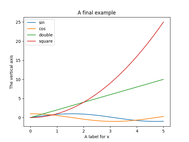
Using our graphing skills, we can now finally plot the graphs of the functions we defined earlier:

# Generally import statements go at the top of the Python file,
# organized in alphabetical order
import math
import matplotlib.pyplot as plt

def response(f, lo, hi, step):
    x_vals = []
    y_vals = []
    x = lo
    while x <= hi:
        x_vals.append(x)
        y_vals.append(f(x))
        x += step
    return x_vals, y_vals

def double(x):
    return 2 * x

def square(x):
    return x ** 2

if __name__ == "__main__":
    sinx, siny = response(math.sin, 0, 5, 0.1)
    cosx, cosy = response(math.cos, 0, 5, 0.1)
    doublex, doubley = response(double, 0, 5, 0.1)
    squarex, squarey = response(square, 0, 5, 0.1)

    plt.figure()
    # connected line
    plt.plot(sinx, siny, label='sin')
    plt.plot(cosx, cosy, label='cos')
    # scattered points
    plt.scatter(doublex, doubley, label='double', color='orange', marker='o')
    plt.scatter(squarex, squarey, label='square', color='green', marker='s')
    # axes and title
    plt.title('A final example')
    plt.xlabel('A label for x')
    plt.ylabel('The vertical axis')
    plt.legend()
    plt.show()
    # display to screen -- remember to exit the graph to finish the program
    print("done")

Running the code above will produce a graph like the one below:

6) Reading and Writing csv Files

Finally, let's talk about one more useful built-in module.

Sometimes the input to your program might be stored in a file. For example, if I am writing a program to process items in my grocery list, and my grocery list lives in a comma-separated values file called grocery_list.csv, it'd be convenient if my program could access the contents of that file. Python can do just that!

The first thing to do in order to use a file is to open it. This is done by invoking the built-in function open

We can open a file in different modes, like read mode or write mode. Since we're just reading from the file for now, we'll tell that to the function open by writing the string 'r'. If my grocery_list.csv file is in the same directory as my Python program¹, I can write

opened_file = open("grocery_list.csv", "r")

opened_file is now an object. With opened_file in hand, we can use the csv module to read the file contents.

We must tell Python that we plan to use it by writing import csv at the top of our file. Then we can create a reader object by calling a function reader which the csv module makes available to us. Our code is now:

import csv

opened_file = open("grocery_list.csv", "r")
reader = csv.reader(opened_file)

reader is an object that allows for iteration. We can print out all the rows in the file, which the reader stores as lists of strings, by looping:

for row in reader:
    print(row)

For a few reasons² (which admittedly aren't likely to be critical for us), if we open a file, we should close it as well, after we're done with it:

opened_file.close()

Since it's very easy to forget to close a file, Python has some great syntactic sugar which automatically does it for us. We can create a with/as block, inside of which the opened file will be open, but outside of which it is automatically closed.

The block doesn't explicitly use the = assignment operator to set the opened_file variable, but it still gives opened_file the same value as before.

Our final program would look like this:

import csv

with open("grocery_list.csv", "r") as opened_file:
    reader = csv.reader(opened_file)
    for row in reader:
        print(row)

import csv

with open("grocery_list.csv", "r") as opened_file:
    reader = csv.reader(opened_file)
    for row in reader:
        print(row)
    for row in reader:
        print(row)

import csv

data_rows = []
with open("grocery_list.csv", "r") as opened_file:
    reader = csv.reader(opened_file)
    for row in reader:
        data_rows.append(row)

# Can now use data_rows multiple times

import csv

groceries = {}

with open("grocery_list.csv", "r") as opened_file:
    csv_reader = csv.reader(opened_file)
    for row in csv_reader:
        if row[1] != "Quantity":
            groceries[row[0]] = int(row[1])
            # note all values are read as strings. If we want a value we
            # read to be treated as a number, we need to cast it to an
            # int or a float!


print(groceries)

Now let's say we wanted to add something to our grocery list, like oranges. While we could append this to our data_rows while running our program, this would not actually change the grocery_list.csv file. Luckily, Python also allows us to write to files. Check out the write.py file below, which does just that:

import csv

data_rows = []
with open("grocery_list.csv", "r") as opened_file:
    reader = csv.reader(opened_file)
    for row in reader:
        data_rows.append(row)

data_rows.append(['Oranges', 3])

# make a new grocery list file
with open('new_grocery_list.csv', 'w', newline='') as csvfile:
    writer = csv.writer(csvfile, delimiter=',')
    for row in data_rows:
        writer.writerow(row)

Note how when we make the new grocery list, we opened the file in 'w' or write mode. Instead of using the csv library to read the file, now we create an object that can write individual rows one at a time. Note that each row is a lists of values, where each element represents the value of a single column.

For more information on the csv library, see the Python documentation.

While working with spreadsheets directly can often be useful, as we'll see in the exercises, using Python to do data analysis can allow us to more easily analyze large amounts of data, especially when it is in a raw or unprocessed format.

7) Summary

In this set of readings, we revisited the details of how Python invokes functions. We also learned the ways in which Python functions are first-class objects. They can be treated just like any other objects in Python: among other things, they can be passed as arguments to functions and can be returned as the result of other functions! We saw assert, which can be used to test programs. And we explored import statements and python packages such as matplotlib, math, and csv which can be used to generate graphs and read and write CSV files.

In next week's readings, we'll investigate one way to use functions: recursion. And we'll talk about strategies for designing large programs.