Readings for Week 3

Licensing Information

The readings for 6.S090 are licensed under a Creative Commons Attribution-NonCommercial-ShareAlike 4.0 International License. You are free to make and share verbatim copies (or modified versions) under the terms of that license.

Portions of these readings were modified or copied verbatim from Think Python 2e by Allen Downey.

PDF of these readings also available to download: reading3.pdf

Table of Contents

This week we're going to learn about a powerful built-in type called a dictionary. We'll also learn how to use Python's extensive standard library, a collection of modules that can add functionality to your programs. Finally, we'll step a bit away from Python specifics, and briefly introduce a useful development tool.

First up: dictionaries. Dictionaries are one of Python's best features; they are the building blocks of many efficient and elegant programs. In some ways, a dictionary is like a list, but more general. Lists and dictionaries are both compound objects, and they are both mutable. In a list, though, the indices have to be integers, whereas in a dictionary they can be (almost) any type.

A dictionary contains a collection of indices, which are called keys, and a collection of values. Each key is associated with a single value. The association of a key and a value is called a key-value pair or sometimes an item.

In mathematical language, we might say that a dictionary represents a mapping from keys to values, so you can also say that each key "maps to" a value. As an example, we'll build a dictionary that maps from English to German words, so the keys and the values are all strings.

Lists in Python are created with square brackets (e.g. new_list = []). Dictionaries, on the other hand, are created with squiggly brackets. For example, we could make an empty dictionary with:

en2de = {}

To add items to the dictionary, you can use square brackets:

en2de['dog'] = 'Hund'

This line creates an item that maps from the key 'dog' to the value 'Hund'. If we print the dictionary now, we see a key-value pair with a colon between the key and value:

print(en2de)  # prints {'dog': 'Hund'}

This output format is also an input format. For example, you can create a new dictionary with three items:

en2de = {'dog': 'Hund', 'cat': 'Katze', 'guinea pig': 'Meerschweinchen'}

If you print en2de, you will see {'dog': 'Hund', 'cat': 'Katze', 'guinea pig': 'Meerschweinchen'}. However, in earlier versions of Python than those we use in this class, you may have seen {'cat': 'Katze', 'dog': 'Hund', 'guinea pig': 'Meerschweinchen'} or {'guinea pig': 'Meerschweinchen', 'dog': 'Hund', 'cat': 'Katze'} — something with the key-value pairs in a different order than specified! In general, you should assume that the order of items in a dictionary is unpredictable¹.

But that's not a problem because the elements of a dictionary are not looked up based on their order; rather, you use the keys to look up the corresponding values:

print(en2de['cat'])  # prints Katze

The key 'cat' always maps to the value 'Katze', so the order of the items doesn't really matter!

If the key isn't in the dictionary, you get an error:

print(en2de['eagle'])  # gives us an error: KeyError: 'eagle'

So far, we've seen that square brackets are used to look up values in a dictionary, and also to add new items to a dictionary. It turns out that they are also used to change an existing mapping. For example, if we wanted our en2de dictionary to store the Swiss dialect German words, we could update our dictionary like so to account for this change:

en2de['dog'] = 'Hundli' 
print(en2de)  # prints {'dog': 'Hundli', 'cat': 'Katze', 'guinea pig': 'Meerschweinchen'}

But we speak High German, so let's put it back:

en2de['dog'] = 'Hund'

Importantly, dictionaries are not limited to containing strings. They can have arbitrary objects as values, and arbitrary immutable objects as keys². We can also mix-and-match, so a single dictionary might have keys and/or values of several different types.

So any of the types we've learned about so far are valid values (including lists, functions, other dictionaries, etc), but certain things cannot be keys into a dictionary (specifically, mutable objects like lists and other dictionaries).

x = [14,7,5]
en2de[x] = 2

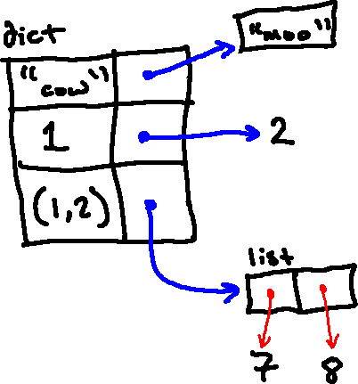
As we've done whenever we've introduced a new type of Python object, we'll learn a way to represent dictionaries in environment diagrams. Note that a dictionary is much like a frame in some ways; it is a mapping between keys and values. So our representation will look very similar: we'll put the keys in the left-hand side of this mapping, and the right-hand side will consist of pointers to the associated values.

For example, the following dictionary:

{'cow': "moo", 1: 2, (1, 2): [7, 8]}

would be represented as follows in an environment diagram:

Beyond the operations above (adding, changing, and looking up key-value pairs), we can also do a number of other interesting operations on dictionaries.

The len function works on dictionaries; it returns the number of key-value pairs:

print(len(en2de))  # prints 3

>>> len(en2de)
3

We also have another useful operation on dictionaries (and, in fact, on many of the other compound objects we've studied) via the in operator.

With dictionaries, the in operator tells you whether something appears as a key in the dictionary (appearing as a value is not good enough).

print('cat' in en2de)  # prints True
print('sandwich' in en2de)  # prints False
print('Katze' in en2de)  # prints False

"in" for Other Sequences

The in operator also works for other kinds of compound objects, as described below:

• element in some_list evaluates to True if any equivalent object to element (compared via ==) exists as one of the elements in the list represented by some_list.
• element in some_tuple behaves the same way.
• some_string in some_other_string behaves differently: it will evaluate to True if the string some_string is a substring of the string some_other_string.

The "not in" operator

Python also provides an operator called not in, which does the opposite check, but is easier to write than the alternative form. So the following two expressions are equivalent:

not needle in haystack  # using the "in" operator and using "not" on the result

needle not in haystack  # using the "not in" operator

Suppose you are given a string and you want to count how many times each letter appears. There are several ways you could do it:

1. You could create 26 variables, one for each letter of the alphabet. Then you could traverse the string and, for each character, increment the corresponding counter, probably using a chained conditional.

2. You could create a list with 26 elements. Then you could convert each character to a number, use the number as an index into the list, and increment the appropriate counter.

3. You could create a dictionary with characters as keys and counters as the corresponding values. The first time you see a character, you would add an item to the dictionary. After that you would increment the value of an existing item.

Each of these options performs the same computation, but each of them implements that computation in a different way.

An advantage of the dictionary implementation is that we don't have to know ahead of time which letters appear in the string and we only have to make room for the letters that do appear.

Here is what the code might look like:

string = 'foo' #whatever string we want to analyze
d = {} #make a new dictionary
for char in string:
    if char not in d:
        d[char] = 1 #we need to add the key to the d
    else:
        oldcount = d[char]
        d[char] = oldcount + 1 #key already exists in d, so increment its value
print(d)

The second line of the program creates an empty dictionary. The for loop traverses the string. Each time through the loop, if the character char is not in the dictionary, we create a new item with key char and the initial value 1 (since we have seen this character once). If char is already in the dictionary, we increment d[char].

If we used 'brontosaurus' as the string, we would print:

{'a': 1, 'b': 1, 'o': 2, 'n': 1, 's': 2, 'r': 2, 'u': 2, 't': 1}

This indicates that the letters 'a' and 'b' appear once; 'o' appears twice, and so on.

Other Operations: "get"

The code above to check whether a key exists in a dictionary, and to use a default value (0 in the example above) if it does not, is a very common pattern. Therefore, Python provides an easier way to accomplish it: get.

To use get, you write it with a key and a default value. If the key appears in the dictionary, get returns the corresponding value; otherwise it returns the default value. For example, working with our dictionary from earlier:

d = {'a': 1, 'b': 1, 'o': 2, 'n': 1, 's': 2, 'r': 2, 'u': 2, 't': 1}
print(d.get('a', 0))  # 1
print(d.get('p', 0))  # 0

string = "foo"
d = {}
for char in string:
    d[char] = d.get(char, 0) + 1
print(d)

If you use a dictionary in a for statement, it traverses the keys of the dictionary. For example, we could print each key and corresponding value of a dictionary:

d = {'a': 1, 'b': 1, 'o': 2, 'n': 1, 's': 2, 'r': 2, 'u': 2, 't': 1}
for char in d:
    print(char, d[char])

and it will produce the following output:

a 1
b 1
o 2
n 1
s 2
r 2
u 2
t 1

This is equivalent to using the dictionary's built-in function .key() which returns an iterable object with all of the keys:

for char in d.keys():
    print(char, d[char])

Again, you should generally not assume that the keys are in a particular order. To traverse the keys in sorted order, you can use the built-in function sorted:

for key in sorted(d):
    print(key, d[key])

produces the following output:

a 1
b 1
n 1
o 2
r 2
s 2
t 1
u 2

If your loop only uses the values in the dictionary, you can loop over the dictionary's .values():

for val in d.values():
    print(val) # prints the values

This is equivalent to the below:

for key in d:
    print(d[key])

You can also loop over both the keys and values at the same time, via .items():

for item in d.items():
    print(item) # prints a tuple (key, value)
    # can access the key via item[0]; the value via item[1]

This is equivalent to below:

for key in d:
    print((key, d[key]))

As we've seen, given a dictionary d and a key k, it is easy to find the corresponding value v = d[k]. This operation is called a lookup.

But what if you have v and you want to find k? You have two problems: first, there might be more than one key that maps to the value v. Depending on the application, you might be able to pick one, or you might have to make a list that contains all of them. Second, there is no simple syntax to do a reverse lookup; you have to search.

Here is code that prints all of the keys in d that map to a value v:

for k in d:
    if d[k] == v:
        print(k)

We now change gears a bit, away from talking about dictionaries and loops. Python provides a large library of other functions and constants which are not available by default, but which can be imported and used within your code. These objects are available in collections called modules.

One common use of imports is to gain access to functions and constants defined in a Python module called math. Before we can use the objects in a module, we need to import them with an import statement, for example:

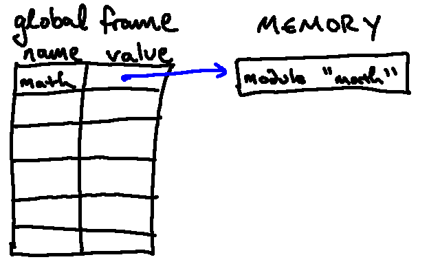
import math

This statement makes a module object in memory and associates it with the name math. In our environment diagrams, we'll denote this as:

We can access functions or constants from within the module using dot notation. For example, to look up and print the constant associated with the number e, we could do the following (after having used import as above):

print(math.e)

To evaluate an expression like this, Python first looks up the name math, finding the module stored in memory. The "dot" (.) then tells Python to look inside that module for something with the name e. In this case, because the math module does indeed contain something called e, it finds that object; so we would see:

2.718281828459045

The math module contains other constants (tau, pi, and others), and it also contains functions, such as sin and log³. We can look up these objects using dot notation as well, and then use them like so:

print(math.sin(3 * math.pi / 4))

import math
print(math.log(82, 3))

Importantly, module objects in many ways can be treated just like any other Python objects: For example, even though it is not a sensible thing to do, we could give another name to the math module after importing it:

import math
foo = math

This would result in the following environment diagram:

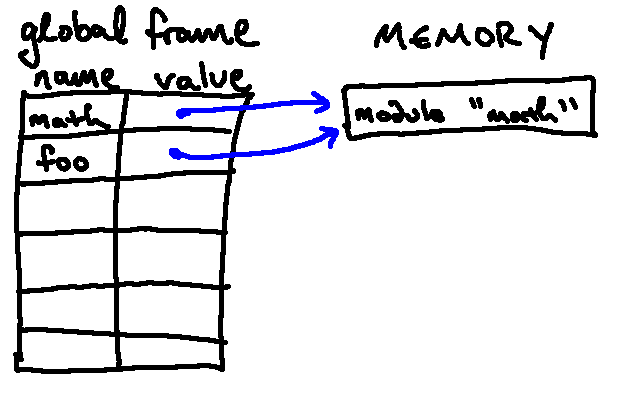
and then we could, for example, look up foo.sin and get the same sin function we would get from evaluating math.sin!

There is a lot of power in the math module, and it turns out that Python has a number of useful built-in modules that we can import from, as well (modules for dealing with strings, with e-mail, with generating random numbers, etc). There are many more that we'll see later.

Reading from csv Files

Now we'll introduce another useful built-in module.

Sometimes the input to your program might be stored in a file. For example, if I am writing a program to process items in my grocery list, and my grocery list lives in a comma-separated values file called grocery_list.csv, it'd be convenient if my program could access the contents of that file. Python can do just that!

The first thing to do in order to use a file is to open it. This is done by invoking the built-in function open ⁴. We can open a file in different modes, like read mode or write mode. Since we're just reading from the file for now, we'll tell that to the function open by writing the string 'r'. If my grocery_list.csv file is in the same directory as my Python program⁵, I can write

opened_file = open("grocery_list.csv", "r")

opened_file is now an object. With opened_file in hand, we can use the csv module to read the file contents. We must tell Python that we plan to use it by writing import csv at the top of our file. Then we can create a reader object by calling a function reader which the csv module makes available to us. Our code is now:

import csv

opened_file = open("grocery_list.csv", "r")
csv_reader = csv.reader(opened_file)

csv_reader is an object that allows for iteration. We can print out all the rows in the file, which the reader stores as lists of strings, by looping:

for row in csv_reader:
        print(row)

For a few reasons⁶ (which admittedly aren't likely to be critical for us), if we open a file, we should close it as well, after we're done with it:

opened_file.close()

Since it's very easy to forget to close a file, Python has some great syntactic sugar which automatically does it for us. We can create a with/as block, inside of which the opened file will be open, but outside of which it is automatically closed. The block doesn't explicitly use the = assignment operator to set the opened_file variable, but it still gives opened_file the same value as before.

Our final program would look like this:

with open("grocery_list.csv", "r") as opened_file:
    csv_reader = csv.reader(opened_file)
    for row in csv_reader:
        print(row)

with open("grocery_list.csv", "r") as opened_file:
    csv_reader = csv.reader(opened_file)
    for row in csv_reader:
        print(row)
    for row in csv_reader:
        print(row)

data_rows = []
with open("grocery_list.csv", "r") as opened_file:
    csv_reader = csv.reader(opened_file)
    for row in csv_reader:
        data_rows.append(row)

# Can now use data_rows multiple times

Modules Beyond the Standard Library

While Python's standard library contains numerous useful modules, there are also modules available outside of the standard library; that is, modules which aren't installed by default with your Python installation. You can import these modules as well, and use them in the same way as above, after installing them on your machine. Usually installing them is a matter of running pip install package_name in a Terminal or Command Prompt, as you did at our kickoff to install numpy, scipy, and matplotlib. (Instructions are here, for reference.)

We now change gears a final time, to introduce Jupyter notebooks.

A Jupyter notebook is a type of document that can contain both code and rich text elements (such as images, equations, and other formatted text). This makes it a useful tool for sharing results of an analysis program, for example, which you may wish to accompany with non-code descriptions or visuals.

Here's a screenshot of a Jupyter notebook:

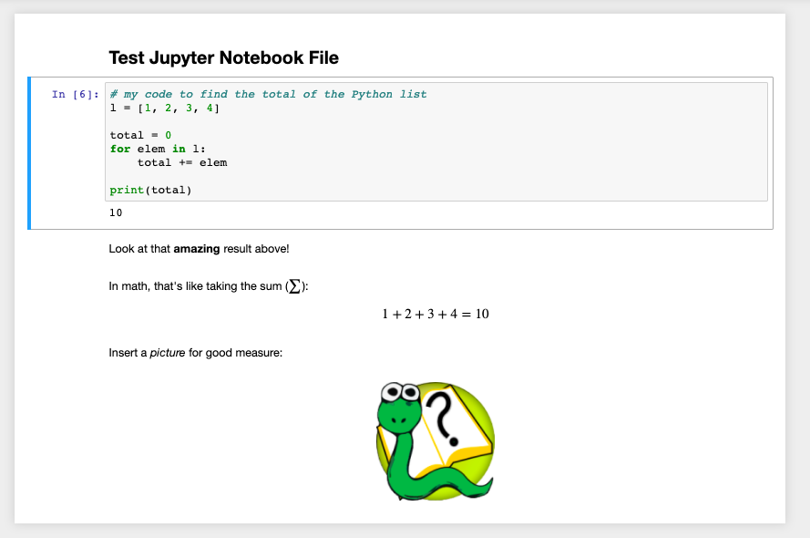
Our goal in this reading is to show you very basic functionality of Jupyter notebooks. There is extensive documentation available here if you'd like to explore further, and we're also happy to answer questions!

Beyond this reading, you will not be required to use Jupyter notebooks in this course. And, in particular, the files you submit to the exercises should still be normal python (.py) files, not Jupyter Notebook (.ipynb) files. However, you will see Jupyter notebooks in other courses.

Installation

Many of you will already have Jupyter installed from your Python installation, like if you installed Anaconda. To check, open a Terminal or Command Prompt, type jupyter notebook, and press enter. It may take a few moments, but it should eventually print a message like "Serving notebooks from local directory" and open a tab in your browser.

If the above does not work, then run the command pip install jupyter (or pip3 install jupyter) in the Terminal/Command Prompt, and try it again. Ask us if you run into issues!

Basics

Running jupyter notebook opens a page in your browser. (Note that the page is not relying on an internet connection, perhaps unlike most pages you view with your browser. Rather, as is the case for all URLs beginning with localhost, the page is getting its content from your own "local" machine.)

The page will look like the dashboard below. Open it now and follow along!

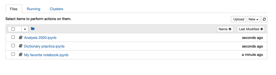
Notice the categories at the top: "Files," "Running," and "Clusters." You will likely live almost exlusively in the "Files" category, which lists all files and folders in the directory in which you ran jupyter notebook. (There may be non-Jupyter-Notebook files listed here, too.)

Here on the dashboard, you can click on an existing notebook to open it, view it, and edit it.

You can also make a new file. Click the "New" dropdown in the top right. Choose to create a new Python notebook⁷. It will open a blank notebook in a new tab:

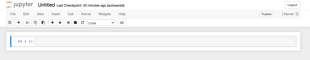
You can click on "Untitled" at the top to change the name of the file.

The new file contains a single cell. Cells are components of Jupyter notebooks. Each cell can contain content of a particular type. For our purposes, there are two types of cells: code, or Markdown. The first cell is by default a code cell. Try typing in a Python expression there. Then, click the "Run" button (this one: ) to executed its contents. You should see the Python result:

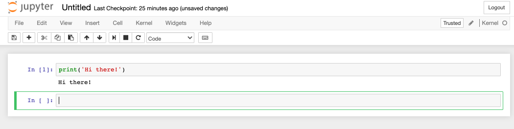
After running the cell, Jupyter automatically gave us a new cell. We could have added a new cell ourselves using the "Add" () button. And we can delete cells with the "Remove" () button.

Let's make this new cell a Markdown cell. In the top menu bar, find the Dropdown that says "Code," and switch it to "Markdown." Markdown is a plain text formatting syntax. In other words, it's a set of rules about how to make text be displayed a certain way. If you've ever written _underscores_ around a word to italicize it, or **asterisks** around a word to make it bold, you've used Markdown! Here's a useful cheat sheet for the Markdown syntax, and there are examples below.

Type some things into your Markdown cell. When you run the cell, you'll see the results of the formatting on your text. For example, this cell:

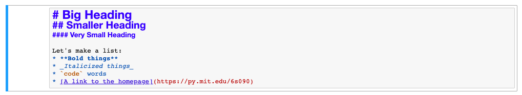
becomes this, after running:

Markdown also supports inclusion of images. In order to include the Python picture in our first example, we moved the python.png file to the same folder as our Jupyter notebook, and included a Markdown cell with the following contents. Note that the path to the image has to begin with "files/," despite the image being in the same directory as the notebook.

To quit Jupyter, close all the browser tabs and press "Ctrl-C" in the Terminal/Command Prompt in which you launched it.

Other Notes

The above should be all you need to know to about Jupyter notebooks for your other courses. Here are some other miscellaneous notes which you may find useful:

• You can share variables and imports across cells. This makes it easy to separate your code into chunks, without having to reinitialize variables or reimport modules.
• The keyboard shortcut for running a single cell while you have it selected is "Shift+Enter"
• To run all the cells, you can choose "Run All" from the "Cell" dropdown menu.
• As noted, you can generally stay almost exclusively in the "Files" category of your dashboard. If, however, you find that code in your notebooks takes quite long to run, you may wish to "Shutdown" some of the running notebooks in the "Running" category.

In this reading, we introduced dictionaries and saw a few sample programs involving them. We also learned how to import python modules, giving us access to the powerful python standard library, and we introduced Jupyter notebooks.

In this set of exercises, you'll get some practice with dictionaries. In the next set of readings and exercises, we will formally introduce a powerful means of abstraction: functions.

Back to exercises