Readings for Unit 4

Licensing Information

The readings for 6.S090 are licensed under a Creative Commons Attribution-NonCommercial-ShareAlike 4.0 International License. You are free to make and share verbatim copies (or modified versions) under the terms of that license.

Portions of these readings were modified or copied verbatim from the very nice book Think Python 2e by Allen Downey.

PDF of these readings also available to download: 6s090_reading4.pdf

Table of Contents

1) Introduction

So far, we have learned about a number of useful tools in Python. We have learned about:

• several types of Python objects that allow us to represent a variety of things in Python's memory (the types we have seen so far include numbers, strings, Booleans, the special None value, and compound objects like lists, tuples, dictionaries and sets); and
• several control flow mechanisms that allow us control over the order in which statements in a Python program are executed (the control flow mechanisms we have seen so far include if/elif/else, and while and for loops).

These are some really powerful tools, and, as you've seen through the exercises, they are enough to accomplish a wide variety of things!¹ However, this week, we'll learn more about an incredibly powerful means of abstraction that will help you manage the complexity as the programs you write become more and more complicated: functions.

Let's start our discussion of functions by considering the following code, which is designed to compute the result of evaluating a polynomial (represented as a list of coefficients) at a particular numerical value:

coeffs = [7, 9, 2, 3] # represents 7 + 9x + 2x^2 + 3x^3
x = 4.2

result = 0
for index in range(len(coeffs)):
   result = result + coeffs[index] * x ** index
print(result)

This is a nice piece of code in the context of a program that requires evaluating a polynomial, but in some sense it isn't as useful as it could be, in that it works only for the values of coeffs and x given above.

It is possible, however, to imagine a larger program that requires evaluating several polynomials. With the tools we have available to us so far, if we wanted to use the code above to this end, we would have to copy the code and paste it to new locations several times. Depending on what our program is doing, we might need to change the variable names coeffs, x, and result to prevent them from overwriting values we had computed for other polynomials. This is a pain! Not to mention, if we find a bug in our implementation, we would have to go back and fix it in every copy-pasted copy we made of this code!

It would be nice to be able to generalize the notion of this computation so that we could perform it on arbitrary inputs as part of a larger program. It turns out that a function, a type of Python object, is a great way to do this!

Functions are arguably the most powerful tool any programmer can have in their toolkit, but it can be a bit complicated to keep track of how Python handles them. As such, we're going to introduce relatively few new topics in this section, so that we can focus on functions, on how Python goes about evaluating code inside a function, and on how they can be used to increase the modularity of the programs we write.

2) Functions

A function is a type of Python object that represents an abstract computation. It can help to think of a function as a little program unto itself, which performs a specific task. Internally, that's what a function really is: it is a generalized sequence of statements that Python can evaluate to compute a result. This is perhaps not the most elegant definition in the world, so let's move on by way of example.

Python comes with several functions built in, and, in fact, we have already seen several examples of functions in Python. For example, we already learned about len, which computes the length of an input sequence. We could use len inside of a program, for example, by evaluating the following expression: len("twine")

In this example, the name of the function we are working with is len. The parentheses indicate that we want to "call" the function², which means to evaluate the sequence of statements it represents. The expression inside the parentheses (here, "twine") is called an argument³ to the function. In this case, the result is an integer representing the length of the argument.

It is common to say that a function "takes" one or more arguments as input and "returns" a result. This result is also called the return value. In this case, len is a function object, and the result of calling it is an int. But, importantly, functions can return values of any type!⁴

We can treat the result of calling a function the same way we would treat any other Python object. For example, we could:

print(len("twine"))  # print the result
x = len("yarn")  # store the result in a variable
y = len("thread") + 27/2  # combine the result with other operations.

2.1) Multiple Arguments

Some functions take more than one argument. To specify this, we separate arguments with commas inside the parentheses associated with a function call. For example, consider Python's built-in round function, which can take two arguments:

print(round(3.14159, 2))  # round returns a number; this will print 3.14

Alternate Forms of Previous Functions

It turns out that two of the functions we have already dealt with have alternate forms that take more than one argument, which may be useful in your programs moving forward:

• If print is given more than one argument, it will print all of its arguments on the same line, separated by spaces. If it is given no arguments (i.e., print()), it will simply make a blank line.
• range has three forms:

  • If range is given a single integer x, the object it returns contains the numbers from 0 to x-1, inclusive.

  • If range is given two integers x and y, the object it returns contains the numbers from x to y-1, inclusive.

  • If range is given three integers x, y, and z, the object it returns contains all values x + i\times z such that x \leq x + i\times z \lt y, in increasing order of i. We can think of z as the step size that we take to go from x to y. This form is commonly used to iterate backwards: range(10, 0, -1).

x = print(7)
print(x)

print(print(print(10)))

10
None
None

2.2) Substitution Model

Before we can go too much farther, we need to think about how Python evaluates functions in our substitution model. In order to evaluate a function call, Python takes the following steps:

• Looks up the value to the left of the parentheses
• Evaluates each of the arguments from left to right
• Calls the function with the results of evaluating the arguments

round(985.654321 + 2.0, len("ca" + "ts"))

round(987.654321, len("ca" + "ts"))

round(987.654321, len("cats"))

round(987.654321, 4)

987.6543

x = 2
z = x(3.0 + 4.0)
print(z)

3) Defining Custom Functions

Using built-in functions or functions imported from Python modules is all well and good, but real power comes from being able to define functions of your own. This is accomplished via a Python statement called a function definition statement, which uses a Python keyword called def.⁵

This is perhaps best seen by example:

def maximum(x, y):
    if x > y:
        z = x
    else:
        z = y
    return z

This statement does two things:

• it creates a new function object in memory, and
• it associates the name maximum with that object in the current frame.

A function definition statement always starts with the keyword def, followed by an arbitrary name for the function. The sequence of names within the parentheses after the function's name are called parameters or, interchangeably, arguments (in this case, x and y), and the function describes a computation in terms of those parameters (as well as, potentially, other values, constants, etc.).

Like many of the structures we have seen, function definitions also have a body (all the code that is indented one level farther than def; in this case, the whole if/else statement). The return keyword, which is only usable inside a function definition, tells Python what the function should produce as its return value when it is called.

Importantly, this statement only defines the function; Python does not run the code in the function body yet! It simply makes an object that represents this function and associates the given name with that object.

3.1) Function Environment Diagrams

As with every new object we've introduced, we'll need a way to represent these objects in memory. Functions need to keep track of three pieces of information, and we'll try to depict all of those in our representation:

1. The names of the parameters to the function, in order;
2. The code in the body of the function; and
3. The frame in which the function was defined.

The following shows an example environment diagram that would result after executing the function definition statement above:

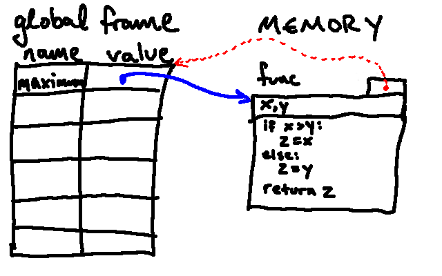
A few notes about this drawing:

• Note that the function definition did two things: it created a new function object, and it bound the name maximum to that object in the global frame.
• The names x,y on the top line of the function object represent the parameters of the function.
• The red arrow points back to the frame in which the function was originally defined (in this case, the global frame).

We can then call this function just as we would with any of the built-in functions (or imported functions) we've seen so far. For example:

a = 7.0
b = 8.0
x = 3.0
y = 4.0

c = maximum(a, b)

We'll now spend some time learning about what happens when this function is called. In the simplest terms, this is what happens:

1. First, Python looks up the name maximum and finds the function object in memory.
2. Next, Python runs the code in the function body with the parameters replaced with the values given (here, the body of the function would be evaluated with x replaced by 7.0 and y replaced by 8.0) until either it reaches a return statement or the end of the body. If a return statement is reached, execution of the function stops and the associated value is returned; if the end of the function is reached (without hitting a return statement), the function returns None.

So after running the code above, c will have value 8.0.

That said, it will be important for us to understand how exactly Python got to that result, and so we'll go into more detail on these steps in the next section. Grab a cup of tea and settle in! This will get complicated, but understanding it is crucial to understanding some of the behaviors we will see from Python in the future! Don't be afraid to re-read multiple times, and, of course, to ask questions if you are confused!

4) Calling Custom Functions

We now examine what happens when a user-defined function is called. We'll go through the example from above. In unit 5's readings, we'll explore more complex examples.

Here is the code (repeated from above) for our example:

a = 7.0
b = 8.0
x = 3.0
y = 4.0

c = maximum(a, b)

(Assume that maximum has already been defined as above)

We know how the first four lines will behave: Python will associate the names a, b, x, and y with the values 7.0, 8.0, 3.0, and 4.0, respectively, in memory, resulting in the following environment diagram:

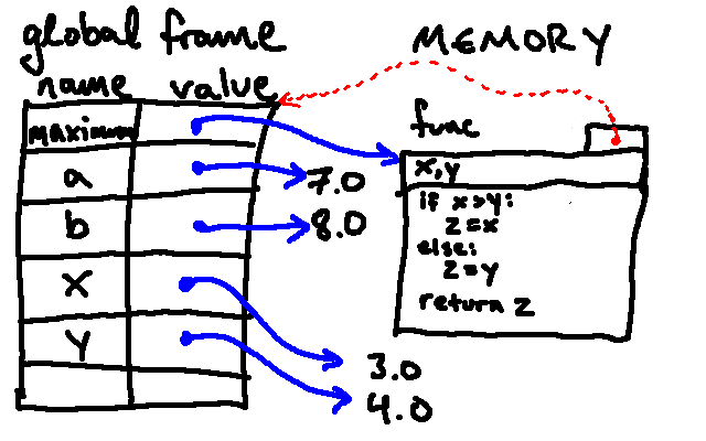
Now we are on to the line where the function call is evaluated. To accomplish this evaluation, Python completes the following steps:

1. As we saw with built-in functions, Python first starts by evaluating the name maximum (finding the function object), followed by the arguments to the function (which evaluate to the 7.0 and 8.0 that a and b, respectively, point to).

2. This is where things get different. Python's next step when calling a user-defined function is to create a new frame. This frame will be similar to the global frame in that it will map names to variables, but these variables will be local to the function (i.e., they will only be accessible inside the function being called).

   Once this new frame is created, Python binds the names of the parameters to the argument that were passed in to the function. From this point on, variable lookups will happen inside this new frame (until the function is done executing).

   This frame also contains a "parent pointer" to the environment in which the function being called was defined.⁶

   Once this step is done, we will have an environment diagram like the following:

   

   As promised, this is a bit complicated. The frame in the bottom-left contains the bindings that exist inside the function. The green arrow represents the "parent pointer."

3. Python then executes the body of the function within this new frame. This means that, if Python looks up x, it finds the value 7.0 (bound in this frame), rather than the 3.0 value that is bound in the global frame. When looking up a variable, if it is not found in the current frame, Python then continues looking for that name in the parent frame before giving up.

   In the process of executing the function body, if Python makes any new assignments, those are also made in the current frame.

   So when our example code assigns a value to the variable z, that binding is made in the current frame. In the course of executing the conditional, we assign z to the same value as y, which results in the following environment diagram:

   

4. When the body is over or a return statement is reached, Python notes the value to be returned. (In the below diagram, the red "return" does not indicate an actual new variables called "return"; rather, it simply indicates the value that is to be returned from the function). Here, the return value was z, which pointed to the 8.0 currently in memory, so that is the value that will be available as the result of calling this function: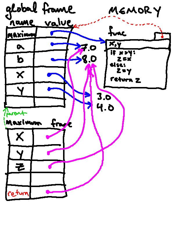

   

   Python then stops executing this function and returns to executing in the frame from which the function was called, after returning the value in question. It also cleans up the new frame it created⁷. In our example from above, the return value is then associated with the name c in the global frame, leaving us with the following: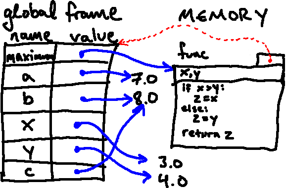

   

4.1) Abstraction

Notice that above, the process of creating the new frame gave us a wonderful feature: the variables inside the function body don't affect the variables outside the function body. This allowed us to call something x inside the function body and not have that cause problems with the thing called x outside the function (when the function is done executing, if we print x, we see the 3.0 that was assigned to x in the global frame)!

This is the real reason functions are so powerful: they offer us a means of abstraction (meaning, once we have defined a function, we can use it knowing only its end-to-end behavior, without worrying about exactly how that behavior was implemented in the function body, what variable names were used, etc.).

4.2) Short Version

Here is the short version of Python's process for calling a user-defined function (again, for details, please see above):

1. Evaluate the arguments. (If an argument is itself a function call, apply these steps to it.)
2. Make a new frame. It stores a pointer to the frame's parent (the frame in which the function was defined).
3. Bind the arguments. In step 1, you already evaluated and simplified the arguments. Now you just have to bind variables to those values in the new frame.
4. Execute the body of the function in this new frame. Depending on what you see, you may be drawing more bindings and/or drawing new frames.
5. Note the return value of the function.
6. When execution has finished, remove the frame and resume execution in the calling frame.

5) More Environment Diagram Examples

Let's look at another environment diagram example. The code below, defines and calls a function named quad_eval, which evaluates the value of a quadratic formula a v^2 + b v + c at a particular value, v.⁸

def quad_eval(a, b, c, v):
    term1 = a * v ** 2
    term2 = b * v
    return term1 + term2 + c

n = quad_eval(7, 8, 9, 3)
print(n)

Use the buttons below to navigate through the process of drawing out the environment diagram for this program. We encourage you to follow along and draw the diagram for yourself alongside us as you're stepping through below!

<< First Step  < Previous Step  Next Step > Last Step >>

Explanations go here.

Now that you've worked through the example above, answer the following question about it:

In step 4 above, when we set up the frame F1 for this function call, we set its parent pointer to be the global frame. For what reason was the parent pointer set this way?

The function we're calling was being called from the global frame.

The function we're calling was originally defined in the global frame.

The name we used to refer to the function, quad_eval, was bound in the global frame.

Something else

Loading...

Another Example

Now that we've talked through the process by which functions are defined and called, we'll take a look at how they play out in a small example. This small program is, admittedly, a little bit contrived... but it should still illustrate how these rules give rise to the behaviors that we expect to see from functions.

Here is the piece of code we'll be considering (note that the names foo and bar don't have any real meaning, but they're conventionally used to refer to functions for which we don't have nicer names, often in silly examples like this):

x = 500

def foo(y):
    return x+y

z = foo(307)

print('x:', x)
print('z:', z)
print('foo:', foo)

def bar(x):
    x = 1000
    return foo(308)

w = bar(349)

print('x:', x)
print('w:', w)

What value will be printed for x on line 8?

Loading...

What value will be printed for z on line 9?

Loading...

What value will be printed for x on line 18?

Loading...

What value will be printed for w on line 19?

Loading...

Now that you have made a guess, let's draw an environment diagram as a way to help us reason about what happens when we run this code; and if we're careful with following the associated rules, we can use the diagram to accurately predict the output of the program above. But this is a complicated example, so grab a cup of tea or coffee and settle in. If you are confused by anything that follows, please feel free to ask for help!

<< First Step  < Previous Step  Next Step > Last Step >>

STEP 1
Before we start running this program, we set up our initial environment structure. Here we have set up our "global frame" (GF), in which our program will be executed.

The next step to be executed is the assignment statement on line 1 (x = 500). What should the diagram look like after that statement has been executed?

STEP 2
Evaluting 500 gives us a new object that represents the integer 500. After creating this object, we associate the name x with it (in the global frame).

The next statement we encounter is a function definition. As mentioned above, Python will do two things here: firstly, it will make a new object to represent this function; then, it will associate that new function with a name (in this case foo).

STEP 3
Here we see the function object itself. Note the three things stored inside of the function: the names of the parameters (in this case, a single parameter called y), the body of the function (return x+y), and a reference to the enclosing frame (i.e., the frame we were running in when we executed this def statement).

Here we have labeled the reference to the enclosing environment with those words, but we will not always write that out.

STEP 4
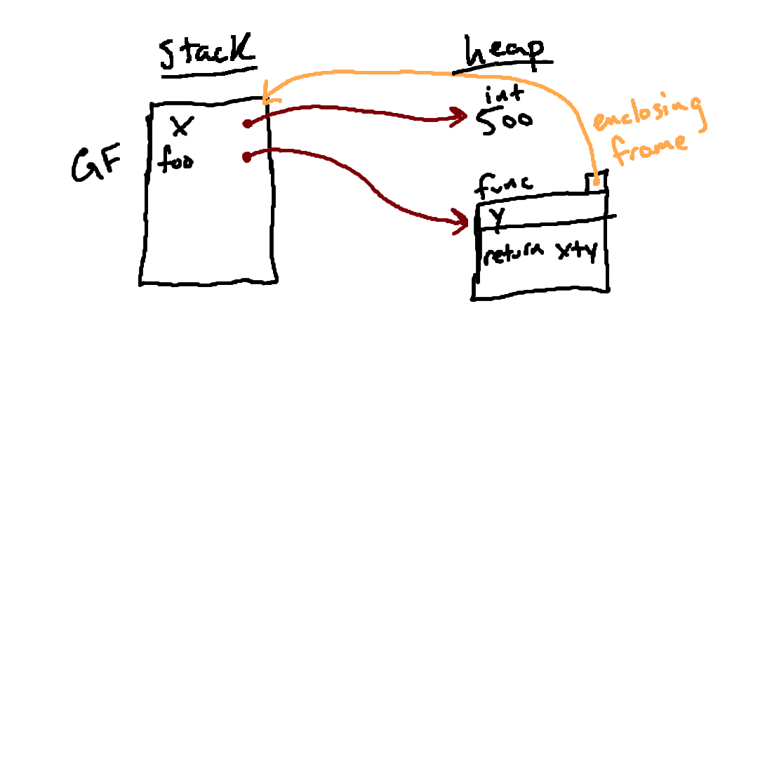
Now we have also associated that function with the name fooin the global environment.

Note that we have not run any part of this function's body yet; we have just stored away the relevant information so that we can eventually call this function.

STEP 5
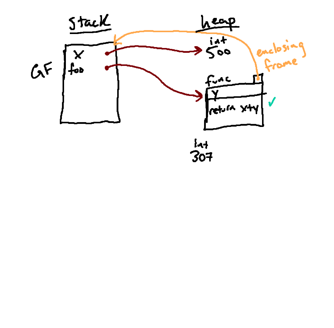
After finishing with the def statement, we are moving on to line 6, z = foo(307). This represents a function call, and so we need to follow the steps outlined under the "Calling a Function" header above.

We start by figuring out what function to call and what to pass to it. In this case, the function we're calling (the thing before the round brackets) is given by the expression foo. Evaluating that name in the global frame, we follow the associated arrow and find the function object on the right (marked with a small green check mark so that we can keep track of it).

Then we evaluate the arguments to the function. In this case, we have a single argument 307. Evaluating that expression produces a new object representing the integer 307.

Once we know what function we're calling and what arguments we're passing in to it, we are ready to proceed with the function call.

STEP 6
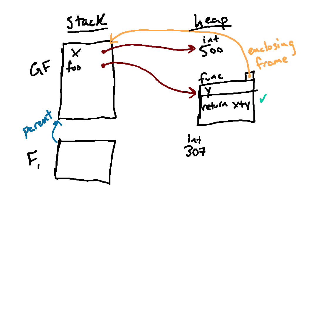
Our next step is creating a new frame to store the local variables associated with this function call. So we have made a new frame here. We also give it a name (just so that it is easier to refer to it), in this case F1.

Note that we have already drawn F1's parent pointer. How did we know that GF was the right parent? When we made F1, we looked at the function we were calling and used its enclosing frame as F1's parent.

Now that we've got our new frame set up, we proceed with our next step: binding the parameters of the function to the arguments that were passed in.

STEP 7
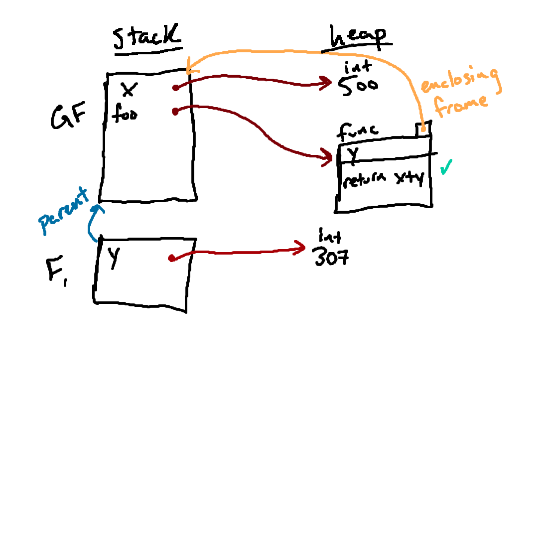
Here we see the end result of binding the parameters of our function to the arguments that were passed in. In this case, the function we're calling is a function of a single parameter (y), and the argument that was passed in is the object we see containing 307.

After this step, we have our local frame all set up, and we are now ready to actually run the body of the function.

STEP 8
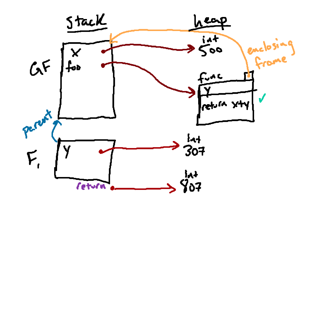
After we've set up the frame associated wth this function call, we proceed by executing the body of the function inside of F1. In this case, the body of the function is return x+y.

Executing return x+y with respect to F1 involves evaluating x and y with respect to F1 and then adding those results together.

Evaluating y with respect to F1, we follow the arrow from y to the associated object, finding the integer 307 that was passed in as argument.

Evaluating x with respect to F1 is a little more complicated, since the name x is not bound in F1. But here we see the nature of the parent pointer. When evaluating a variable name in a given frame, if we don't find the name bound in that frame, we will follow the frame's parent pointer and look for the name there. If we find the name there, the associated object is the result. If we still don't find the name, we follow the next parent pointer; and we keep doing this until we either find the name we're looking for, or we run out of frames to look in. In this case, we don't find x in F1, so we follow its parent pointer and look for x in GF, where we find the associated value of 500.

Once we have those two pieces, we add them together, producing a new object representing the integer 807. This new object is the return value from our function call, which we will sometimes denote as above. Our function call is now done, and we need to look back and remember how we got here. In this case, we started this function call in the process of evaluating line 6, where our goal was to associate the result of the function call with the name z in the global frame.

STEP 9
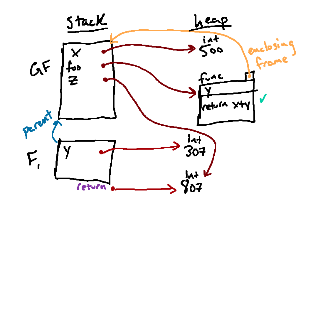
Here we see the result of that assignment. At this point, we are done with the function call, and we can clean up all of the machinery that we used to figure out how the function call behaved and move back to executing code in the global frame. The result of that cleanup will be shown in the next step.

STEP 10
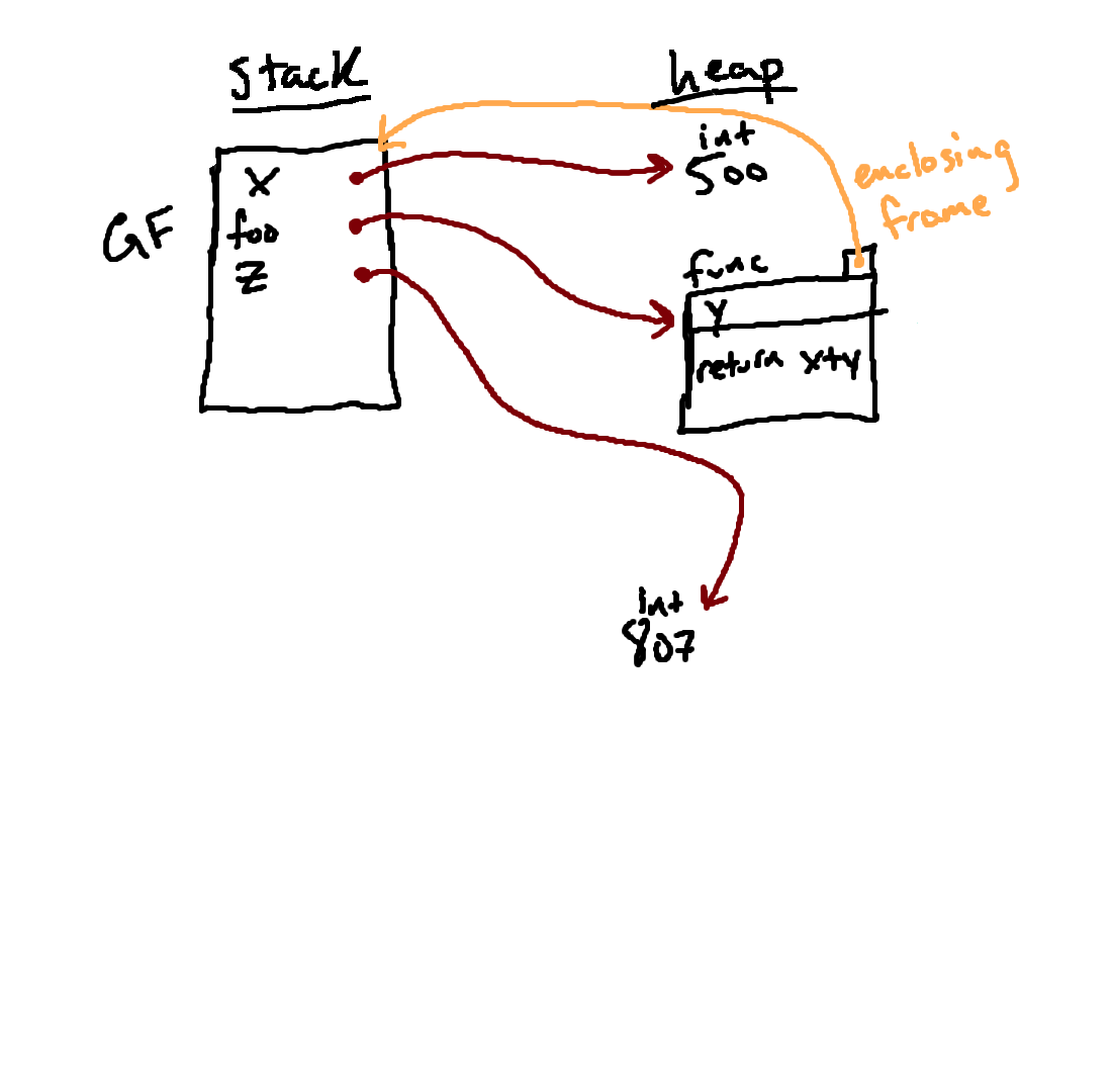
Here we see the result after line 6 has been executed. Next, we hit three print statements. Following the arrows in our diagram, we can now see that x is associated with 500 and z is associated with 807; so we can predict that those are the values that will be printed for x and z. But an important question remains: what will be printed for foo?

Even though it may seem strange at first, we can determine what will be printed for foo in the exact same way that we figured out what to print for x and z: by following the arrow in our diagram from the name foo. In this case, we find the function object on the right side of the diagram, which is what Python will print.

Python prints this in a somewhat strange way, but it's trying its best. It prints out a little representation that includes the function object's location in memory, something like <function foo at 0x7f30d9080040>, where the exact number on the right side will be different each time we run the program.

Importantly, what we are printing when we print(foo) is the function object itself, not the result of calling that function. Line 10 does not cause foo to be called; we simply look up the name foo and print the associated object.

Ultimately, we see something like the following as the output of lines 8-10:

x: 500
z: 807
foo: <function foo at 0x7f30d9080040>

Now, we are ready to move on to our next statement, the second def on line 12.

STEP 11
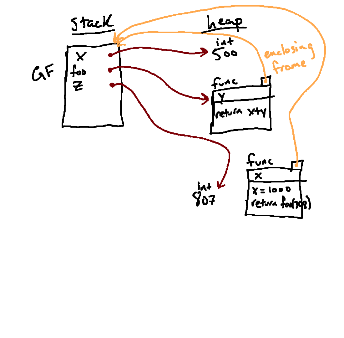
We follow the same rules when executing this def statement as we did before, and the first part of that process results in a new function object, shown in the diagram above. Note again that we have not run any of the code in the body of this new function yet; we are just storing it away to be called later.

STEP 12
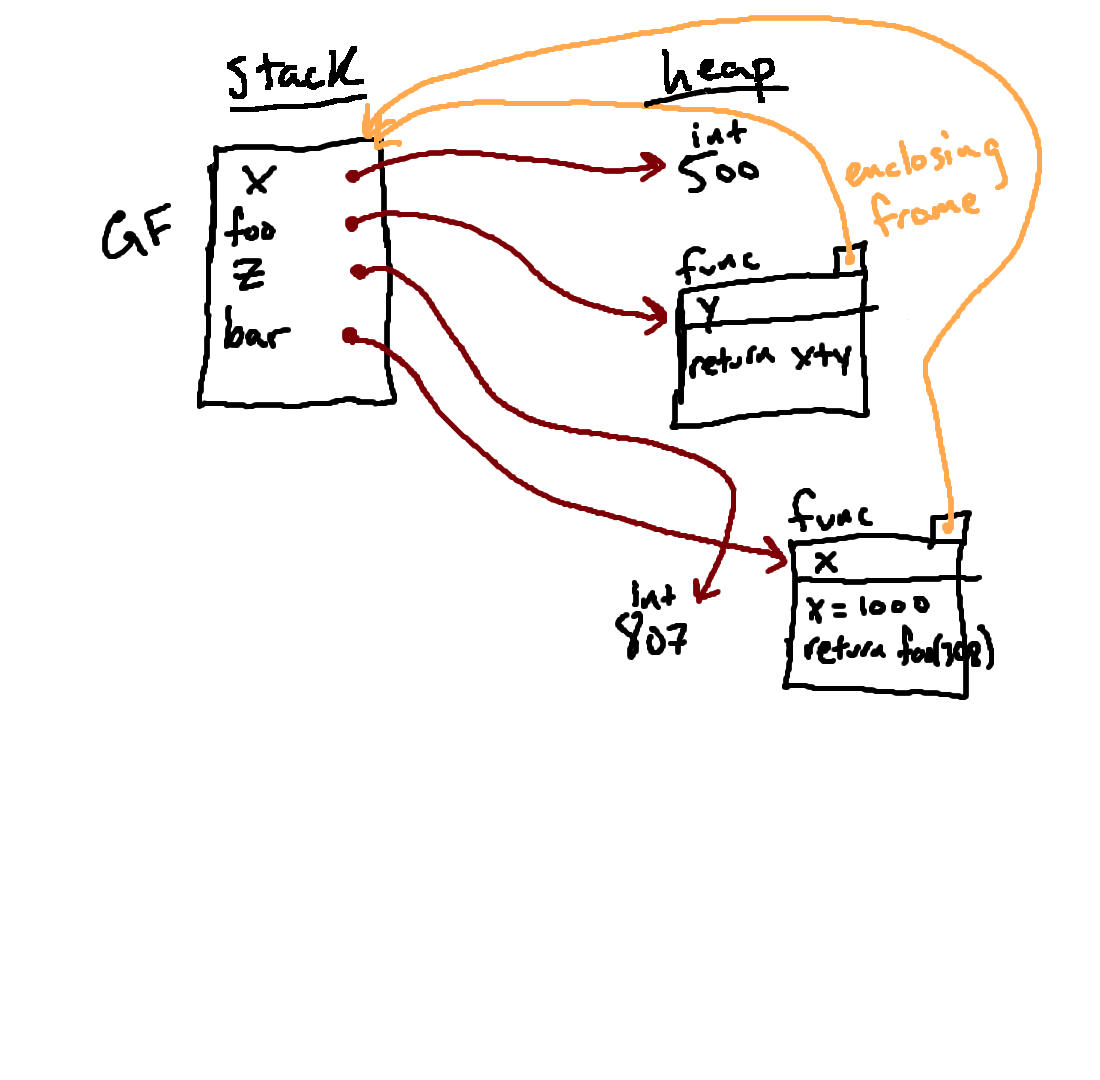
The def statement also associates the name bar with this function, in the global frame. The end result is shown in the diagram above.

With that, we are done with evaluating the def statement that starts on line 12, and we are ready to move on to the next statement, the assignment on line 16.

STEP 13
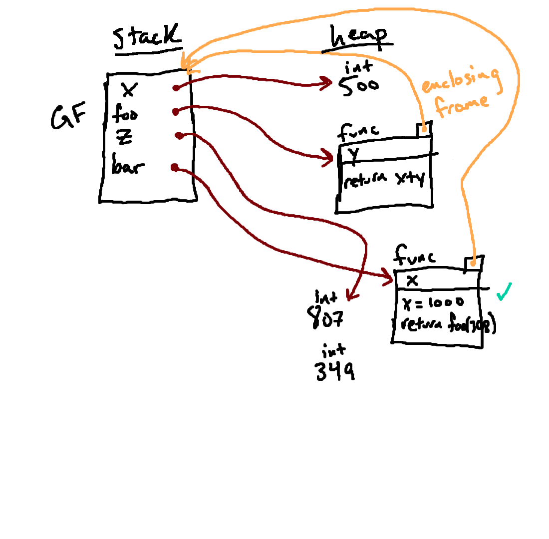
Evaluating the assignment statement on line 16 involves first evaluating the expression on the right-hand side of the equal sign, which is a function call. We start that process by determining what function we're calling and what arguments we're passing in to it.

In this case, the function we're calling is given by bar, and a single argument 349 is given. So we evaluate the name bar, finding the function object indicated with the green checkmark above; this is the function we're going to call. And evaluating 349 produces a new object representing the integer 349, which is the object we are passing in to the function.

Once we know what function we're calling and what we're passing as inputs, we can proceed with the function call using the rules described earlier.

STEP 14
We start by making a new frame to store this function's local variables. Above, we've made this frame and labeled it as F2. Note that F2 has a parent pointer to our function's enclosing frame.

After we have created the frame, our next step will be to bind the parameters of the function to the objects passed in as arguments; the result of this process will be shown in the next step.

STEP 15
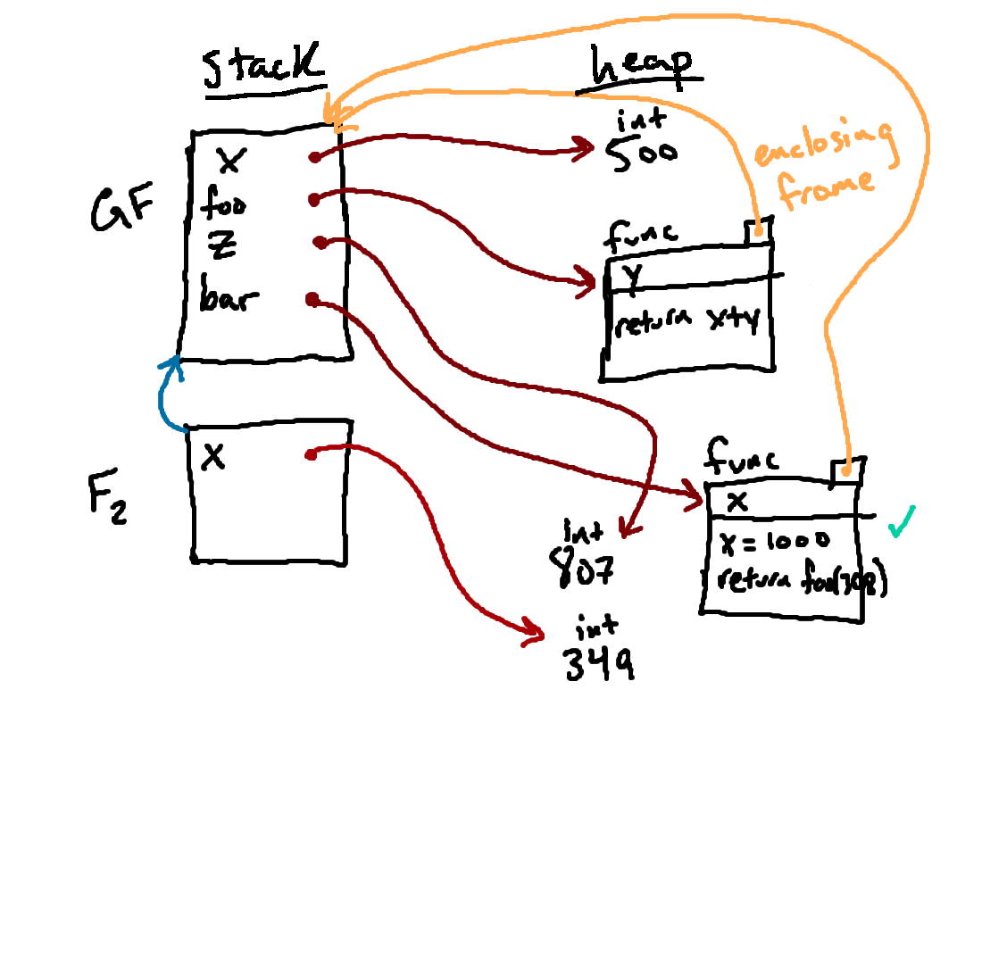
Here, we show the result of binding the name x to the value 349 inside of our new frame F2.

I think it is important to note here that this binding did not affect the value associated with the name x in the global frame. Even though x refers to 349 in F2, x still refers to the value 500 in the global frame. And since we will ultimately evaluate the body of this function inside of F2, referring to x in the function will not find the global binding of x.

This setup (where each function call gets its own frame to store its local variables) is generally really nice and quite powerful, in that it allows us to call the parameters of our functions (and other local variables inside of our functions) by any names we wish, without needing to worry about accidentally messing up the variable bindings in other frames.

Anyway, once we have made that binding, we are ready to execute the body of the function inside of F2. And so the next statement we encounter is x = 1000, which we evaluate with respect to F2. Can you predict what the result will look like? We will show it in the next step.

STEP 16
Since we were executing x = 1000 with respect to F2, we modify the arrow from x inside of F2. Note again that the global binding of x is unaffected. At this point, we're done with x = 1000, so we can move on to the next statement.

STEP 17
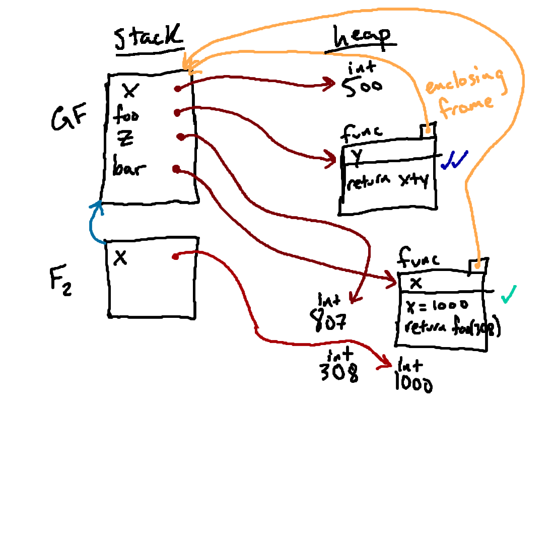
Remember that at this point, we are still executing the body of our function inside of F2. And the next statement we encounter is return foo(308). This is another function call! So what do we do?

Conveniently, even though we are now going to be two function calls deep, we evaluate this second function call in precisely the same way we evaluated the first one, by following the rules laid out earlier on this page. And so the first thing we need to do is to determine what function we're going to be calling and what arguments we're going to pass in. But there is a little bit of subtlety here that we need to be careful of.

Because this function call is being made from F2, figuring out what function to call involves looking up the name foo inside of F2. We don't find the name foo there, so we follow the parent pointer and look in the global frame, where we find that the name foo is bound to the function object that now has two small blue checkmarks next to it; so that's the function object we'll be calling.

Then we evaluate the argument and get a new integer 308, which has been drawn in above as well. And, now that we know what function we're calling and what arguments to pass in, we can proceed with actually calling the function. Our first step will be to make a new frame for this new function call.

STEP 18
Here we have drawn in our new frame (called F3), but we're actually not quite done with that part yet because we have not yet given this frame a parent pointer. **Please take a moment and try to predict**, given the rules we have outlined here, where should F3's parent pointer go?

STEP 19
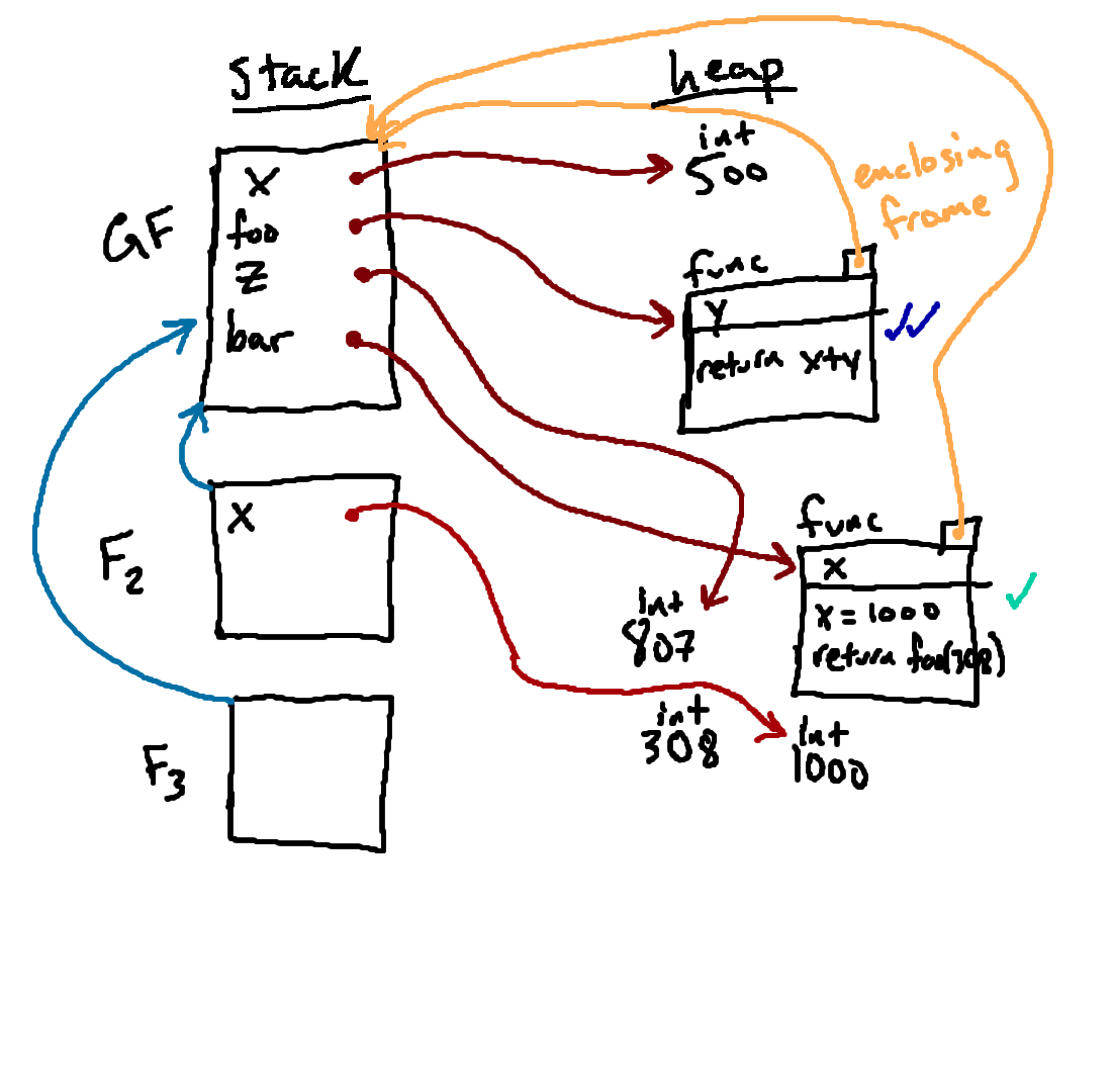
The key rule for determining a new frame's parent pointer is: what is the enclosing frame of the function we're calling? In this case, we're calling the function drawn toward the top of the diagram (with the two blue checks next to it, which is referred to as foo in the global frame); and that function's enclosing environment is GF, so that's where our new frame's parent pointer goes.

Importantly, this is true even though we made this function call from F2! What matters for determining this structure is not where we're making the call from, but rather where the associated function was originally created. This may seem like a strange rule at first, but it leads to a lot of nice properties that we will discuss in more depth during class.

And now that we've set up our new frame, we can move on to our next step, binding the parameters of the function to the arguments that were passed in.

STEP 20
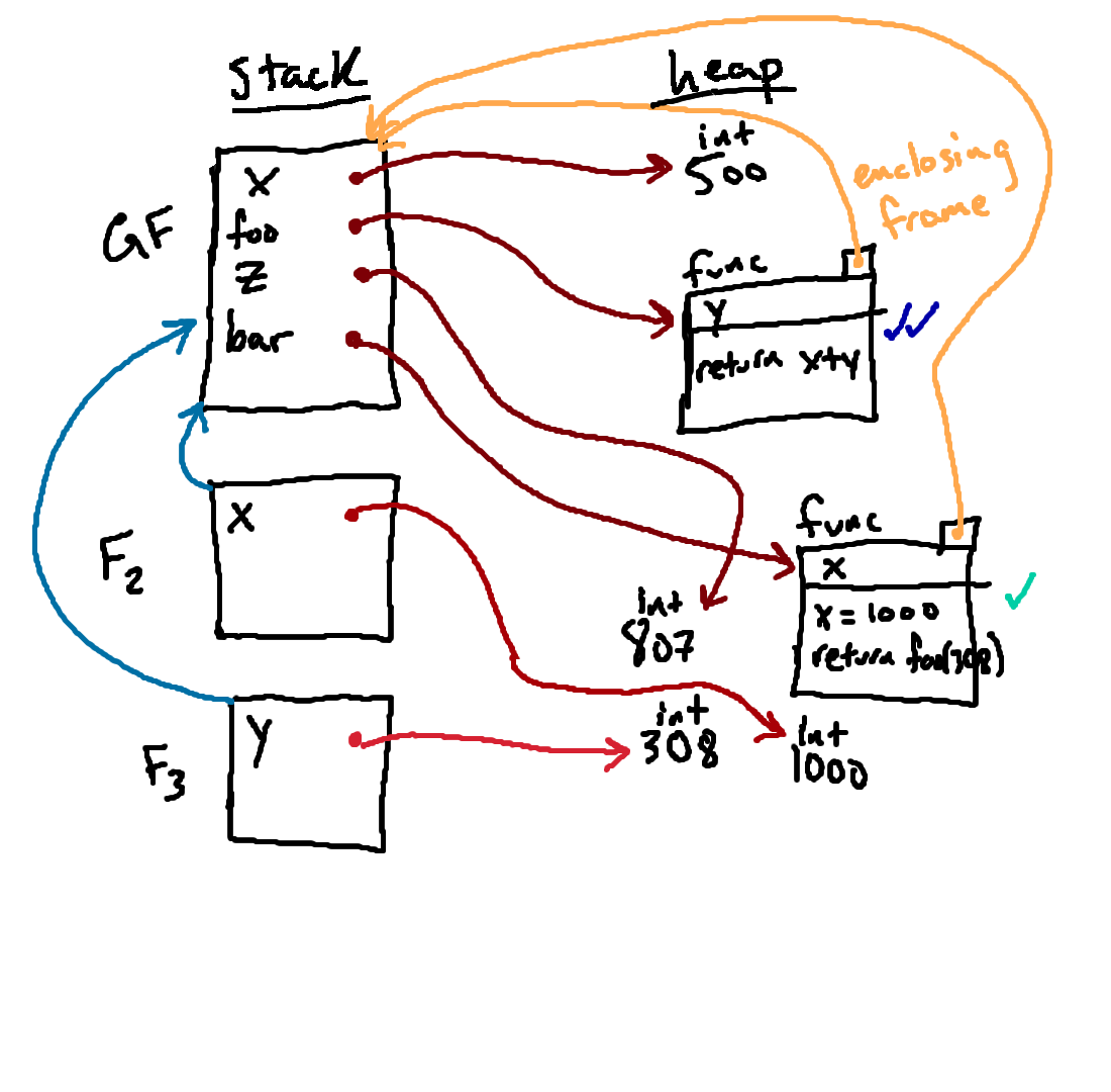
The function we're calling is a function of a single parameter called y, and so inside of F3, we bind the name y to the 308 that was passed in. Having done so, we are ready to execute the body of the function inside F3.

STEP 21
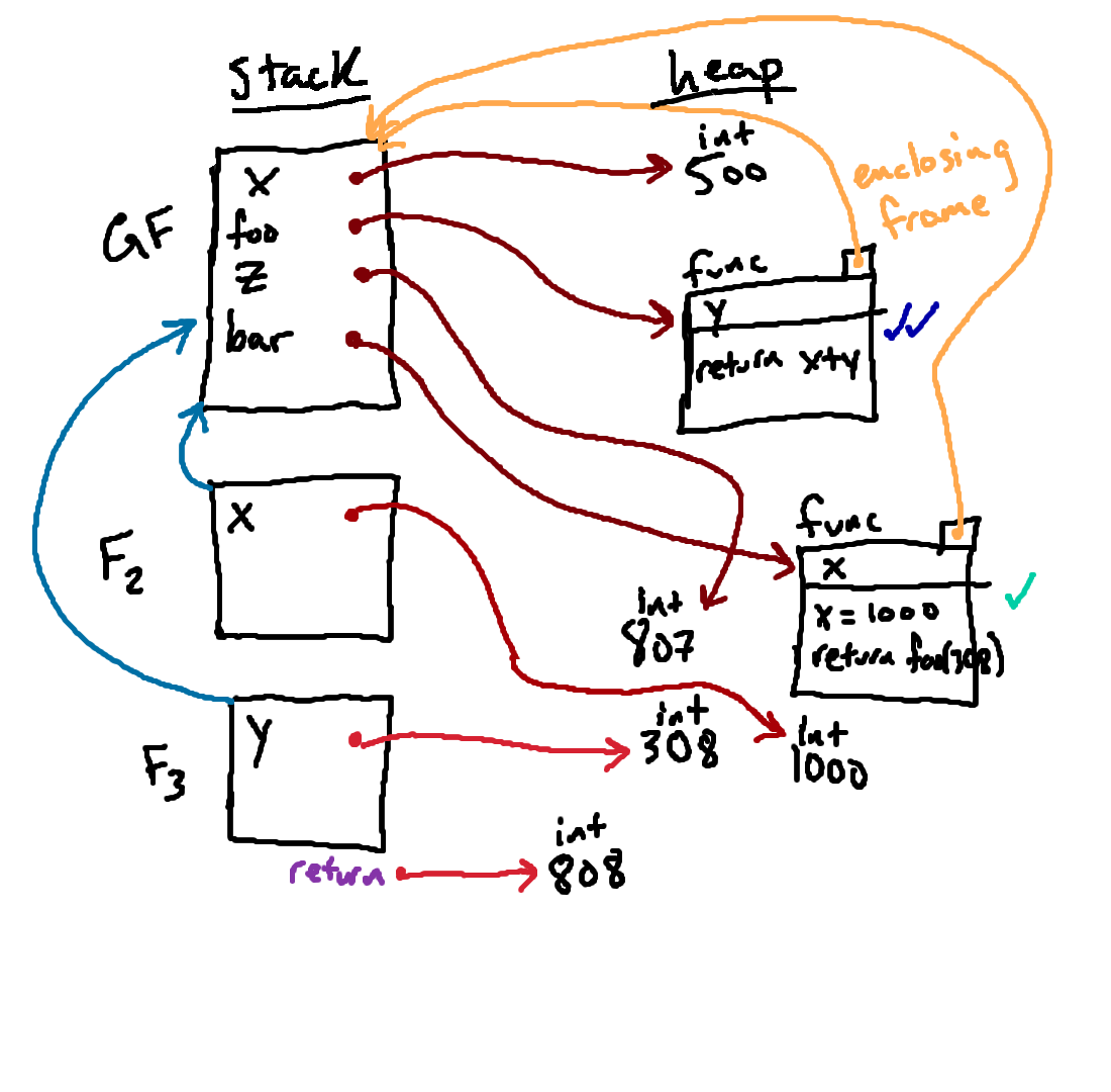
Evaluating the body of the function with respect to F3 involves evaluating both x and y with respect to F3 and then adding the results together to produce the return value of this function call.

Evaluating y with respect to F3 is relatively straightforward: y is bound in that frame, and so we follow its arrow to find the 308 that we passed in as an argument.

Evaluating x with respect to F3 is more involved. We look for x in F3, but we don't find it there, so what do we do next? We follow F3's parent pointer and look for x there. So, importantly, we find the value 500, to which x is bound in the global frame (and not the 1000 to which x is bound in F2).

Adding these values produces a new value 808, which will be our return value.

Now we need to think a little bit. How did we get to this function call, and where should we return back to? Remember that we started this function call in the process of figuring out what to return from our original call to bar. So we'll jump back to that point in the execution, with our new 808 value in hand.

STEP 22
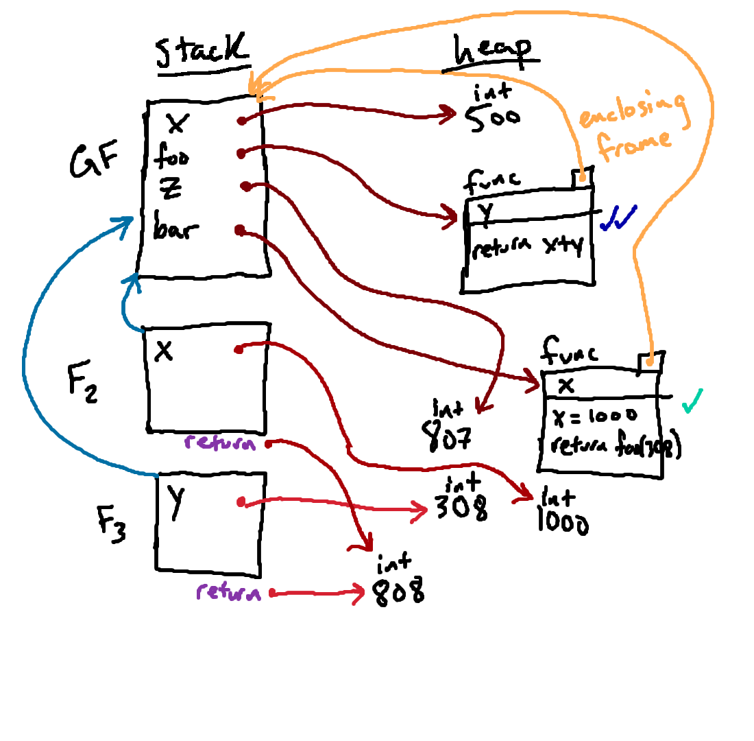
Since the line we had been executing in F2 was return foo(308), we're simply going to take the result of that function call (the 808 we just figured out) and mark it as the return value from F2, which has been reflected above.

At this point, we are also done with that second function call. So on the next step, we'll clean up some of the machinery that we created purely for determining that result.

STEP 23
And we also need to remember: how did we come to be calling bar in the first place? That is, now that we have the output of the function call, where do we return to?

We first got here by executing w = bar(349) in the global frame. So that's where we'll go next, binding the name w to 808 inside of the global frame.

STEP 24
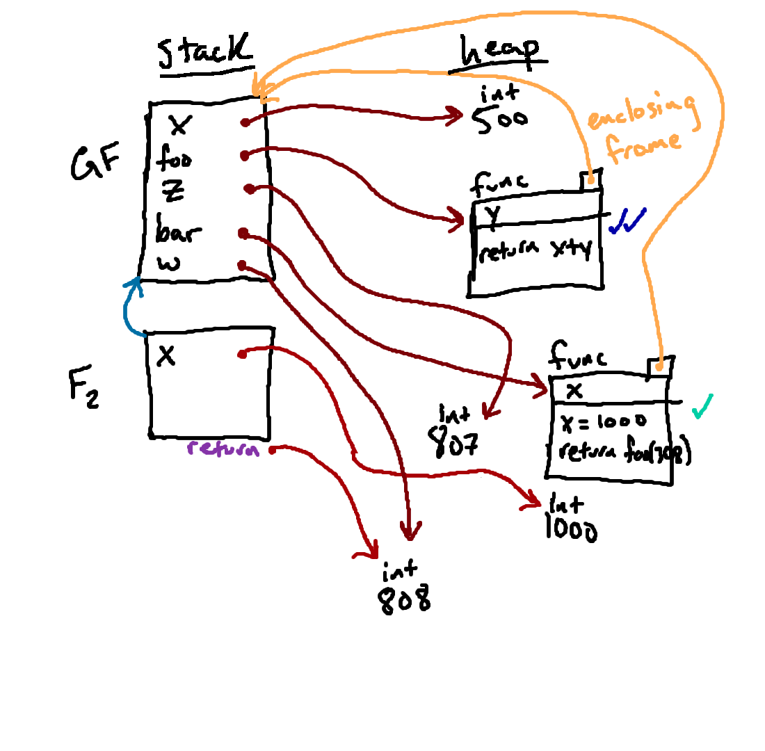
Phew, that was quite a journey! But now we're done with executing line 16 in our original program!

At this point, we can clean up F2, since we're done with that function call, leaving us with one final diagram.

STEP 25
Now the only thing left to do is to figure out what prints when lines 18 and 19 are run. Tracing the arrows from x and w from the global frame, we find 500 and 808 (respectively), and so those are the values that will be printed:

x: 500
w: 808

After the value 808 has been returned from F2, we no longer have a need to keep F2 around, and so it (as well as the integer 1000 that was only reachable from F2) will be garbage collected, leading to the final diagram.

STEP 26
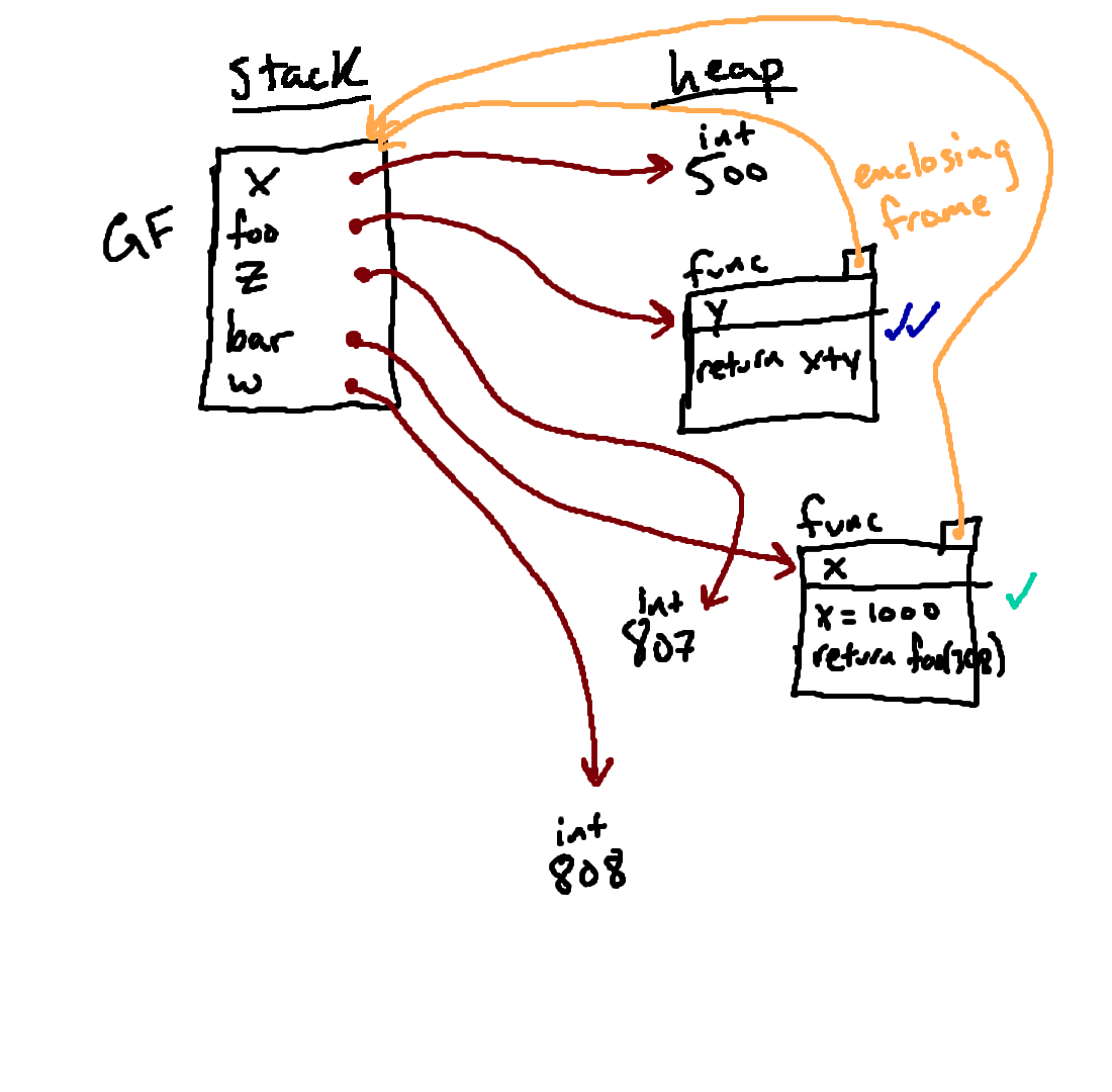
This diagram represents the state of memory at the end of our little program. Notice that the value of 808 that we got from calling our function is still available to us, via the name w in the global frame.

x = 500

def foo(y):
    return x+y

z = foo(307)

print('x:', x)
print('z:', z)
print('foo:', foo)

def bar(x):
    x = 1000
    return foo(308)

w = bar(349)

print('x:', x)
print('w:', w)

One last question for this section: imagine adding x = 2000 to line 5 of the program above and running it again. Which of the following printed values would be different from running the code without that change?

x

z

foo

w

Loading...

If you're unsure of why this answer is what it is, think about how things would change in terms of our environment diagrams. And, of course, if you're stuck, please don't hesitate to ask for help!

6) Built-Ins

Now that we have talked about the notion of multiple frames, we can clear something up about Python's built-ins. We have talked a lot now about how Python looks up the values associated with variable names, and you may have wondered how Python found the built-in values.

How did Python know what function to call when we referenced print? It is true that print and the other built-ins do not exist in the global frame. Rather, we can think of the global frame itself as having a parent pointer to a special "built-ins" frame: when Python looks up a name in the global frame and doesn't find it, it then looks in this special "built-ins" frame before throwing a NameError.

This is how the lookups for, for example, print and len proceed: Python first looks for them in the global frame. Since it doesn't find them there, it looks in the built-ins frame, where it finds them.

Failed variable lookups also proceed in this same way. Say we made a typo and were accidentally looking up the value pritn. In looking this up, Python would first look in the global frame; when it doesn't find pritn there, it would then look in the built-ins frame; and when it doesn't find pritn there either, it will give up and raise a NameError.

7) Print vs. Return

In general, print statements are useful for displaying information to the user, and return statements allow the results of function calls to be stored and passed around within the program, which turns out to be quite useful since you can then look up (or even print) those values again later.

One important difference between print statements and return statements is that once Python reaches a return statement inside a function it immediately stops and exits the function after returning the value. While one function can have multiple print statements that display multiple lines to the screen, return statements are considered a 'hard stop' to the function.

For example, consider the outputs of the following two functions:

def without_return():
    print("without return")
    print("this line gets printed")

def with_return():
    print("with return")
    return "STOP"
    return "this line never runs"
    print("this line never gets printed")

without_result = without_return()
'''   the above line results in the following output:
without return
this line gets printed
'''
print(without_result)  # None


result = with_return()
'''   output:
with return
'''
print(result) # STOP

It is also important to note that in the absence of a return statement, all functions by default return None. For example, consider this function that returns 'positive' if a number is greater than 0:

def is_positive(x):
    if x > 0:
        return 'positive'

result = is_positive(5)
print(result) # prints 'positive'
result2 = is_positive(0)
print(result2) # prints None

Just like print allows you to display multiple values, return statements can also output multiple values:

def divide(dividend, divisor):
    # calc the quotient and remainder of dividing two numbers
    return dividend // divisor, dividend % divisor

result = divide(10, 3) # returns a tuple
print(result) # (3, 1)
print("result is", result[0], "remainder", result[1]) # result is 3 remainder 1
num, remainder = divide(19, 4)  # unpacking the returned tuple
print(num) # 4
print(remainder) # 3

Unlike print, return statements do not need round brackets. If we want to return multiple values, we simply separate them by a comma. If you recall from a couple of units ago, this creates a tuple, which we can clearly see when we print out the result. To access the different returned values, we can simply index into the result, or unpack them into separate variables, as shown above.

7.1) Return to Refactoring

For an example of why using return statements are useful, consider the following problem which we solved earlier in the course:

def simple_full_packages(order, package_limit):
    '''
    Calculate the number of full packages that can be delivered, assuming near
    infinite inventory.

    Inputs:
        order (int) - number of items requested
        package_limit (int) - number of items that can fit in a shipment
          container

    Returns:
        The integer number of completely filled packages.
    '''
    if package_limit == 0:
        num_packages = 0  # avoid Division by 0 error
    else:
        num_packages = order // package_limit

    return num_packages


def num_packages(order, package_limit):
    '''
    Calculate the fewest number of packages that would be required to ship
    all items in an order.

    Inputs:
        order (int) - number of items requested
        package_limit (int) - positive number of items that can fit in a
                                shipment container

    Returns:
        The integer number of packages required.
    '''
    if package_limit == 0:
        num_boxes = 0  # avoid Division by 0 error
    else:
        num_boxes = order // package_limit

    if package_limit*num_boxes < order:
        num_boxes =  num_boxes + 1
    return num_boxes

if __name__ == "__main__":
    # Local testing -- feel free to add your own tests as well!
    print("testing simple_full_packages:")
    print(f"Got {simple_full_packages(10, 0)=}, expected 0")
    print(f"Got {simple_full_packages(10, 3)=}, expected 3")
    print(f"Got {simple_full_packages(5, 5)=}, expected 1")

    print("\ntesting num_packages:")
    print(f"Got {num_packages(10, 1)=}, expected 10")
    print(f"Got {num_packages(10, 3)=}, expected 4")
    print(f"Got {num_packages(10, 5)=}, expected 2")

Notice how the conditional logic is very similar for both functions. In fact, the only difference is a single if statement in num_packages. Because we used return statements instead of print, we can refactor our code as follows, to make it simpler and more concise:

def simple_full_packages(order, package_limit):
    '''
    Calculate the number of full packages that can be delivered, assuming near
    infinite inventory.

    Inputs:
        order (int) - number of items requested
        package_limit (int) - number of items that can fit in a shipment
          container

    Returns:
        The integer number of completely filled packages.
    '''
    if package_limit == 0:
        num_packages = 0  # avoid Division by 0 error
    else:
        num_packages = order // package_limit

    return num_packages


def num_packages(order, package_limit):
    '''
    Calculate the fewest number of packages that would be required to ship
    all items in an order.

    Inputs:
        order (int) - number of items requested
        package_limit (int) - positive number of items that can fit in a
                                shipment container

    Returns:
        The integer number of packages required.
    '''
    num_boxes = simple_full_packages(order, package_limit)

    if package_limit*num_boxes < order:
        num_boxes =  num_boxes + 1
    return num_boxes

Now instead of repeating code, num_packages can use simple_full_packages to calculate the initial number of boxes, and then decide whether a partially full box will be needed.

Code that is simple, concise, and easy to read tends to be both easier to understand and debug. That is why refactoring, the process of revising code to have better style (e.g., descriptive variable names, better high-level comments, consistent spacing), reduced repetition, and less complexity, is an important programming skill that we will continue to practice this week.

8) Why Functions?

To close this section, here are some reasons for using functions:

• Creating a new function gives you an opportunity to name a group of statements, which makes your program easier to read and debug.
• Functions can make a program smaller by eliminating repetitive code. Later, if you make a change, you only have to make it in one place.
• Dividing a long program into functions allows you to debug the parts one at a time and then assemble them into a working whole.
• Well-designed functions are often useful for many programs. Once you write and debug one, you can reuse it.

9) Extras: Syntactic Sugar

Before closing fully, we briefly describe some of Python's "syntactic sugar" to which you've been exposed. Wikipedia explains that syntactic sugar is "syntax ... that is designed to make things easier to read or to express. It makes the language 'sweeter' for human use: things can be expressed more clearly, more concisely, or in an alternative style that some may prefer."

Last week, we saw a lot of examples of syntactic sugar in the form of ternary statements, comprehensions, and the built-in functions min, max, sum and sorted. This week we're going to dive into one more useful piece of syntax that we've been using throughout the course but haven't explained: f-strings.

9.1) String formatting

Sometimes we want to print a combination of text and variables. For example, say we were a grocery store that wanted to display the cost of an item a user selected. With what we know about type-casting and string concatenation we could accomplish this as shown in the example below:

item = 'bread'
cost = 1.99
print("The " + item + " costs $" + str(cost) + ".")
# "The bread costs $1.99."

But what if we wanted to print the cost of five different items? It would be a pain to make sure all the + signs and quotation marks were in the right places. That's why more recent versions of python have introduced more convenient ways of formatting strings.

One particularly useful string formatting method is called the f-string. For example:

print(f"The {item} costs ${cost}.")
# "The bread costs $1.99."

Placing an f at the beginning of the string lets python know to format it so that any value enclosed in curly brackets is evaluated, cast to a string, and then automatically concatenated in the right place.

Using an = sign before the closing curly brackets indicates that you want to display both the code as a string, and the result of evaluating that code. For example:

nums = [1, 2, 3, 4, 5]
print("len(nums) = " + str(len(nums)))

Can be more concisely written with the following f-string:

nums = [1, 2, 3, 4, 5]
print(f"{len(nums) = }")

An older python string formatting method that you might encounter in the "wild" uses % signs to act as a placeholder for a value.

print("The %s costs $%g." % (item, cost))
# "The bread costs $1.99."

The %s indicates that a string value will be inserted, %g means a floating-point number will be inserted. At the end of the string, the values are listed in order. You can find more information about formatting data types using the % notation in python's documentation.

So far, we've used f-strings to help us manually check our code to see if it's getting the expected result. In future units, we'll learn about other tools we can use to get Python to test our code for us!

10) Reading and Writing csv Files

Finally, let's talk about one more useful built-in module.

Sometimes the input to your program might be stored in a file. For example, if I am writing a program to process items in my grocery list, and my grocery list lives in a comma-separated values file called grocery_list.csv, it'd be convenient if my program could access the contents of that file. Python can do just that!

The first thing to do in order to use a file is to open it. This is done by invoking the built-in function open

We can open a file in different modes, like read mode or write mode. Since we're just reading from the file for now, we'll tell that to the function open by writing the string 'r'. If my grocery_list.csv file is in the same directory as my Python program⁹, I can write

opened_file = open("grocery_list.csv", "r")

opened_file is now an object. With opened_file in hand, we can use the csv module to read the file contents.

We must tell Python that we plan to use it by writing import csv at the top of our file. Then we can create a reader object by calling a function reader which the csv module makes available to us. Our code is now:

import csv

opened_file = open("grocery_list.csv", "r")
reader = csv.reader(opened_file)

reader is an object that allows for iteration. We can print out all the rows in the file, which the reader stores as lists of strings, by looping:

for row in reader:
    print(row)

For a few reasons¹⁰ (which admittedly aren't likely to be critical for us), if we open a file, we should close it as well, after we're done with it:

opened_file.close()

Since it's very easy to forget to close a file, Python has some great syntactic sugar which automatically does it for us. We can create a with/as block, inside of which the opened file will be open, but outside of which it is automatically closed.

The block doesn't explicitly use the = assignment operator to set the opened_file variable, but it still gives opened_file the same value as before.

Our final program would look like this:

import csv

with open("grocery_list.csv", "r") as opened_file:
    reader = csv.reader(opened_file)
    for row in reader:
        print(row)

import csv

with open("grocery_list.csv", "r") as opened_file:
    reader = csv.reader(opened_file)
    for row in reader:
        print(row)
    for row in reader:
        print(row)

import csv

data_rows = []
with open("grocery_list.csv", "r") as opened_file:
    reader = csv.reader(opened_file)
    for row in reader:
        data_rows.append(row)

# Can now use data_rows multiple times

import csv

groceries = {}

with open("grocery_list.csv", "r") as opened_file:
    csv_reader = csv.reader(opened_file)
    for row in csv_reader:
        if row[1] != "Quantity":
            groceries[row[0]] = int(row[1])
            # note all values are read as strings. If we want a value we
            # read to be treated as a number, we need to cast it to an
            # int or a float!


print(groceries)

Now let's say we wanted to add something to our grocery list, like oranges. While we could append this to our data_rows while running our program, this would not actually change the grocery_list.csv file. Luckily, Python also allows us to write to files. Check out the write.py file below, which does just that:

import csv

data_rows = []
with open("grocery_list.csv", "r") as opened_file:
    reader = csv.reader(opened_file)
    for row in reader:
        data_rows.append(row)

data_rows.append(['Oranges', 3])

# make a new grocery list file
with open('new_grocery_list.csv', 'w', newline='') as csvfile:
    writer = csv.writer(csvfile, delimiter=',')
    for row in data_rows:
        writer.writerow(row)

Note how when we make the new grocery list, we opened the file in 'w' or write mode. Instead of using the csv library to read the file, now we create an object that can write individual rows one at a time. Note that each row is a lists of values, where each element represents the value of a single column.

For more information on the csv library, see the Python documentation.

While working with spreadsheets directly can often be useful, as we'll see in the exercises, using Python to do data analysis can allow us to more easily analyze large amounts of data, especially when it is in a raw or unprocessed format.

11) Summary

In this reading, we (mainly) introduced functions. Importantly, we also talked about defining new functions of your own creation as a means of abstracting away details of a particular computation so that it can be reused. We spent a good deal of time and effort focusing on how defining and calling these functions fits in to our mental models of Python (substitution model and environment diagrams). In unit 5, we'll solidify this understanding of functions further, with more examples, and we'll introduce some more related function features.

In this set of exercises, you will get more practice with simulating the evaluation of functions and with defining functions of your own. You will also get the chance to practice using string-formatting and reading and writing files, which is useful for data analysis and processing, among other things.

Next Exercise: Fun with Functions

Back to exercises