Readings for Week 2

Licensing Information

The readings for 6.S090 are licensed under a Creative Commons Attribution-NonCommercial-ShareAlike 4.0 International License. You are free to make and share verbatim copies (or modified versions) under the terms of that license.

Portions of these readings were modified or copied verbatim from the very nice book Think Python 2e by Allen Downey.

PDF of these readings also available to download: reading2.pdf

Table of Contents

In the last set of readings, we introduced several types of Python objects, as well as models of how Python evaluates expressions and how it manages storing and looking up variables. We also introduced our first means of controlling the order of the evaluation of statements in a program through conditional execution.

In this reading, we will introduce and explore some new types of Python objects, and we'll see how to fit these new types into our existing framework. We'll also introduce some very powerful new control flow mechanisms.

Before we dive into this assignment's new material, you may wish to review some of the readings and exercises from last week (and, in particular, check the results of the manual grading, including my comments which you can see on the individual assignment pages, if you have not yet). Almost everything introduced in this reading will build on ideas from the last one.

In the last set of readings, we saw that we could display characters to the screen verbatim by enclosing them in quotation marks in a print statement. For example, the following will display hello, python! on the screen:

print("hello, python!")

But at the time, we didn't talk much about what this statement actually meant in terms of our mental model of Python. In this section, we'll start to clarify this a bit by introducing a new Python type into our mental model: strings.

A string is a type that represents a sequence of characters¹. In Python, this type is given the name str. It turns out, also, that it is fine to use either double quotes (") or single quotes (') to enclose strings.² So the Python expression "yarn" evaluates to a string, and so does 'twine'.

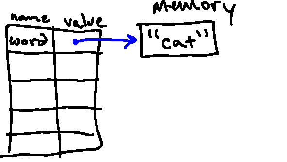
Because strings are actually a type of Python object, it turns out that we can do more than just print them! We can, for example, store a string in a variable:

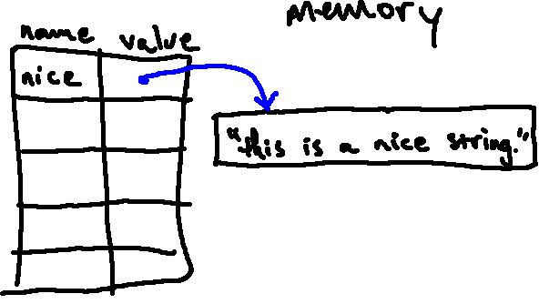
nice = "This is a nice string."

We can think of this the same way we thought of other variable assignments:

• Python will start by evaluating the value on the right side of the = symbol (which, in this case, results in a string).
• It will then store this string in memory, and associate the name nice with it.

Much like we did with int and float objects, we can denote strings in our environment diagrams by simply writing their value, though it may be a good idea also to draw a box around a string so that it's clear that it is a single object. Running the above code snippet, for example, would result in the following environment diagram:³

Once we have the string stored in a variable, we can include the variable in other expressions. For example, after making the definition above, we could print that string with:

print(nice)

This will look up the variable name nice in the global frame; doing so, it finds the string that is stored in memory, which it then displays.

favorite_animal = "dog"
favorite_language = "python"
print(favorite_animal)
print(favorite_language)

favorite_animal = "dog"
favorite_language = "python"
print("favorite_animal")
print("favorite_language")

Operations on Strings

We saw in the last set of readings that the type of an object is important for determining the kinds of operations we can perform on that object. For example, we could perform arithmetic with int and float objects, but not so with NoneType objects. Similarly, we can perform some kinds of operations on strings. We'll come back to this idea more later on, but for now, let's explore the meaning of the + operator as it relates to strings.

print("I'm adding this string" + "to this string")

Try Now:

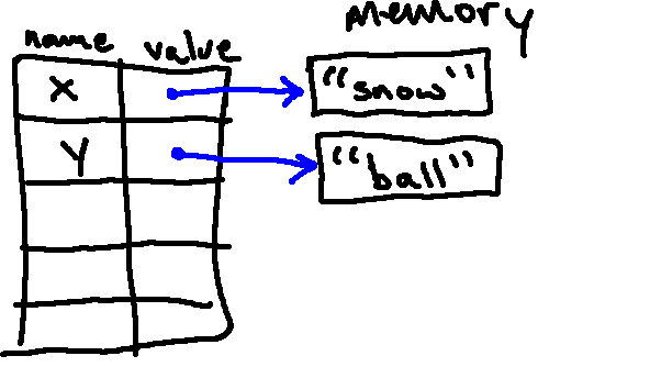
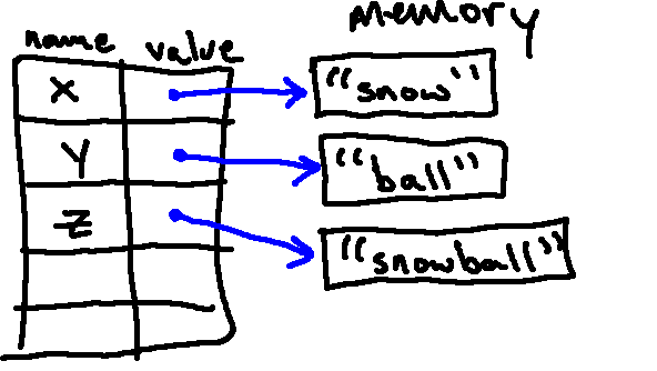
Draw an environment diagram that shows the result of running the following short program, and predict what it will print:

x = "snow"
y = "ball"

z = x + y

x = "basket" + y

print(z + " " + x)  # the middle string contains a single "space" character

Show/Hide

After executing the first line, we have the object "snow" in memory, and the name x associated with it:

After the following line, we have a second object, "ball", in memory, and the name y associated with it:

In the process of evaluating the third statement, Python looks up x (finding "snow") and y (finding "ball"), and concatenates them to form a new string, "snowball". This object is stored in memory, and the name z is associated with it:

Next, we replace the definition of x with the result of evaluating "basket" + y. This evaluation gives us the new string "basketball", which we then associate with x. After we do this, there are no references left to our original "snow" object, so it is garbage collected, giving us the following final diagram:

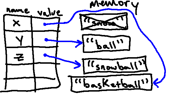
The final line contains a print statement, and we can use our substitution model to determine the value that is printed:

• z + " " + x (Loading z gives us...)
• "snowball" + " " + x (Concatenating the first two terms gives us...)
• "snowball " + x (Loading x gives us...)
• "snowball " + "basketball" (Concatenating these two strings gives us...)
• "snowball basketball"

And so the value that is printed is "snowball basketball".

print("cat" * 20)

Converting Between Types

In the last set of readings, we saw that we could convert between int and float objects (for example, with int(7.8) or float(6)).

It is also possible to convert between strings and numeric types, provided we are dealing with strings in a particular form. For example:

• str(6.0) will give us the string "6.0".
• int("2") will give us the integer 2.
• float("7.8") will give us the float 7.8.

Strings are an example of a compound type: they are sequences of characters. Sequences in Python have a number of interesting operations associated with them. We'll start by exploring these in the context of strings, and then generalize to other kinds of sequences.

Extracting Contained Elements

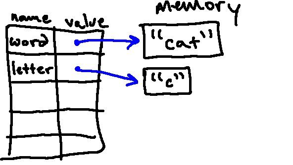
You can ask Python for one character from a string with the bracket operator. For example, try the following:

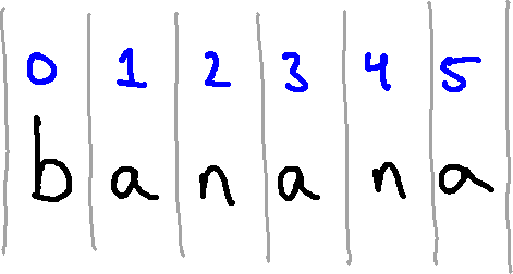
fruit = "banana"
letter = fruit[1]
print(letter)

The second statement selects character number 1 from fruit, stores it in memory, and associates the name letter with it. The expression inside the brackets (in this case, 1) is called an index. The index, which must be an integer, indicates which character in the sequence you want.

But, running the code above, you might not get the answer you expect!

Most people would expect character one from "banana" to be "b". But in Python (as in many programming languages), we actually start counting at 0 rather than at 1⁴.

So the indices from 0 to 5 are associated with the letters in this string as shown below:

It is perhaps also worth noting that you can also index from the end of a string. The index -1 is associated with the last character in a string, -2 with the next to last, and so on. So we really have two indices associated with each character:

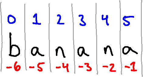
Trying to access an index other than one of those numbers (in this case, integers between -6 and 5, inclusive) results in an error.

We will now introduce two more incredibly useful types of sequences: tuples⁵ and lists.

Tuples

Tuples are sequences like strings, with the important distinction that, while strings are limited to containing only characters, tuples can contain arbitrary objects (integers, floats, Booleans, None, or even other tuples!).

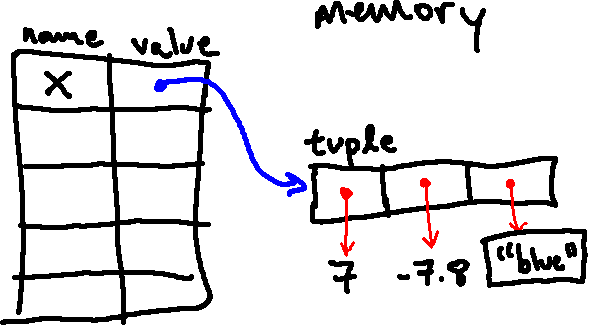
A tuple is specified as a comma-separated sequence of arbitrary objects, usually wrapped in parentheses. For example, the following is a tuple containing three different objects:

x = (7, -7.8, "blue")

We can perform many of the same operations on tuples that we could on strings. For example:

• we can index into a tuple (x[1] gives us -7.8)
• we can use + to concatenate two tuples (x + (1, 2, 3) gives us (7, -7.8, "blue", 1, 2, 3))
• we can compare two tuples using ==

We also need a way to represent tuples in our environment diagrams, to model how Python actually handles them in memory. We will model the above tuple (7, -7.8, "blue") with the following kind of drawing:

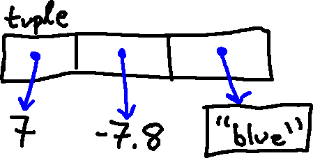
We'll draw it as a box, with the label "tuple" (so that we can keep track of types), with several references to other objects. You can think of these references as being very similar to the mappings we have already considered, from names to objects.

So after evaluating the line of code above (x = (7, -7.8, "blue")), we will have the following environment diagram:

Let's examine what happens when we index into x. Consider, for example, running the following code:

print(x[-1])

Python first looks up x in the global frame. Doing so, it follows the pointer from x and finds the tuple object in memory. Then, it looks up index -1 inside of x. This is the last "slot" in x, and so, following that pointer, we find the string "blue".

Notice here that x[-1] is still a string, and so anything we can do to any other string, we can do to x[-1]. This includes indexing into it! So we could try the following:

print(x[-1][2])

When evaluating x[-1][2], Python will first look up x (finding the tuple in memory). Then it will look up index -1 inside of that tuple (finding the string "blue"). Finally, it will look up index 2 of that string (finding "u"). So this line above with print a u to the screen.

Try Now:

Try drawing an environment diagram for the following code:

a = 1
b = 2
c = 3

x = (c, b, a)
y = (3, 2, 1)

What is different about how the two tuples are represented in memory?

Show/Hide

After executing the first three lines, our environment diagram looks like this:

Then, when creating the first tuple, Python figures out what objects are associated with the locations in the tuple by looking up a, b, and c. As such, the entries in the tuple point to the same integer objects as a, b, and c:

However, when creating the second tuple, Python figures out what objects are associated with the locations in the tuple by evaluating 1, 2, and 3. As such, the entries in the tuple point to different integer objects:

Try Now:

Note that tuples can contain any kind of Python object, including other tuples. So we could have had our last line instead say: y = (3, 2, x). How would the final environment diagram differ if we made this change?

Show/Hide

Here is the resulting environment diagram (notice that the only change is that the last location in the y tuple points to the same tuple as x):

If we had executed this code, how would Python evaluate y[2][0]?

Show/Hide

Python would start by evaluating y and finding a tuple. It would then look up index 2 in that tuple, finding the other tuple, where it then looks up index 0, finding value 3 (the same 3 that is associated with variable c).

Lists and Mutability

The last type of sequence we will introduce today is one of the most useful built-in types, the list. Lists are almost the same as tuples, with one exception that has big potential consequences.

Like strings or tuples, lists are sequences. Like tuples, lists can contain arbitrary Python objects. Unlike strings or tuples, however, lists are mutable; this means that they can be changed after they are created. In this section, we'll examine the effects of this difference.

The syntax for creating lists is similar to the syntax used for creating tuples, except that it uses square brackets instead of round brackets.

For example, we can create some lists as follows:

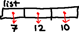
dogs = ['Lab', 'Boxer', 'Poodle']
numbers = [42, 123]
another_list = [7, 12, 10]
empty = []  # we can also make a list that contains no elements!

We will represent lists in environment diagrams similarly to how we represented tuples, but we will mark them clearly as lists. For example:

With a tuple, we would get an error on the last line below:

my_tuple = (1,2,3)
print(my_tuple[0]) # looking up elements is fine -- no error yet
my_tuple[0] = 12

Specifically, we would see the error message: TypeError: 'tuple' object does not support item assignment.

However, if we used a list instead, we could modify the elements contained in the list!

dogs = ['Lab', 'Boxer', 'Poodle']
dogs[2] = 'Pincher'
print(dogs)

['Lab', 'Boxer', 'Pincher']

Try Now:

Draw an environment diagram for the following code, and predict what will be displayed to the screen when the following program is run. Run your code to verify; the results may be surprising!

a = [7, 12, 10]
b = [4, 5, 6]

c = a

print(a)
a[0] = 8
print(a)
print(b)
b[-1] = "cow"
print(b)
print(a)
c[1] = 3.14

print(a)

Show/Hide

After the first two lines are executed, our environment diagram should look like this:

Then, importantly, when we run the next line (c = a), the names c and a both refer to the exact same list object in memory (this does not make a copy of the list), as indicated below:

Then we print a, which will print the current value of a, which is [7, 12, 10]. The next line changes the value to which a[0] points, so we are left with:

Then we print a again, which will print the updated value of a, which is [8, 12, 10]. Then we print b, which will print the current value of b, which is [4, 5, 6]. The next line changes the value to which b[-1] points, so we are left with:

Then we print b again, which will print the updated value of b, which is [4, 5, "cow"]. Then we print a, which will print the current value of a, which is [8, 12, 10]. The next line changes the value to which c[1] points, so we are left with the following:

Importantly, because a and c are both associated with the same list in memory, looking up a will also see the updated value! So when we print a, we see [8, 3.14, 10] In the end, the whole program printed the following:

[7, 12, 10]
[8, 12, 10]
[4, 5, 6]
[4, 5, "cow"]
[8, 12, 10]
[8, 3.14, 10]

Adding Items to a List

Another common way to mutate a list is not by changing one of the elements in a list, but adding a new element to the end of the list. This is accomplished via append. For example:⁶

x = [5, 8, 3, 2, 1]
print(x)
x.append(7)
print(x)

This will print:

[5, 8, 3, 2, 1]
[5, 8, 3, 2, 1, 7]

Note that, unlike concatenating two lists together, this will not make a new list. Rather, it will modify the list in memory with which x is already associated. Although we sometimes have to be careful with it (because of the kinds of issues we saw above), modifying an existing list in memory is almost always substantially faster than making a new list via concatenation.

Because lists can contain arbitrary Python objects, we could use append to add any object to a list.

x.append("a string!")
x.append((7, 8, 9)) # a tuple

Try Now:

What will be printed after the following piece of code is executed?

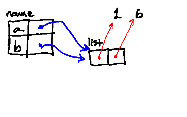
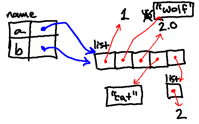
a = [1]
b = a
a.append(6)
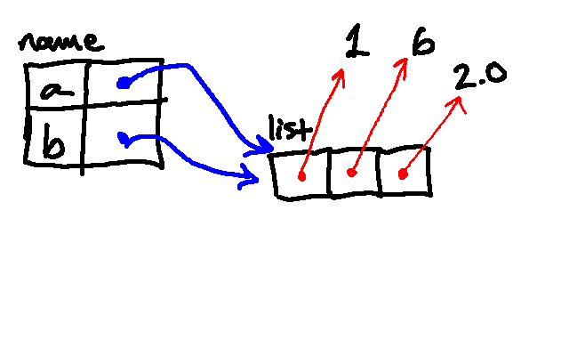
a.append(2.0)
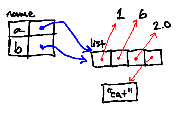
a.append("cat")
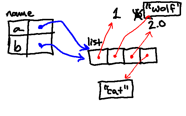
a[1] = "wolf"
a.append([2])
a = [4]
print(a)
print(b)

Show/Hide

The end result is that the following two values are printed:

[4]
[1, 'wolf', 2.0, 'cat', [2]]

In order to see why this is the case, let's simulate using an environment diagram. The first line creates a list containing a single element, a 1, and associates the name a with it:

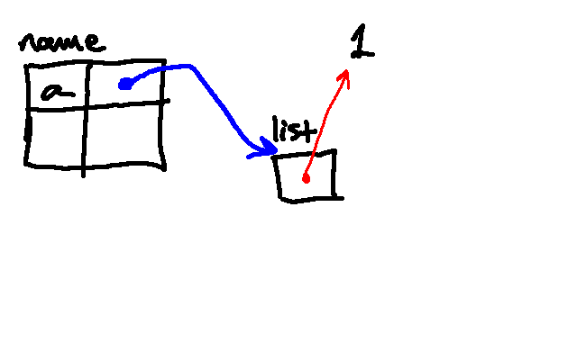
The next line associates the name b with the same list in memory.

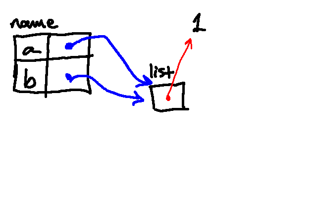
Python then looks up a and modifies the list by appending a 6 to it. Note that, because a and b are two different names for the same object in memory, the value associated with b is also changing!

Then we append 2.0 to the same list:

Then we append the string "cat":

The next line then replaces the element at index 1 in the list with "wolf":

The next line then appends a list containing the number 2 to the list associated with the name a. (Notice here is an example of a list contained within another list.)

Next, we reassign a to be associated with a list containing a single 4. Note that this did not change the binding of b, which is still associated with the original list.

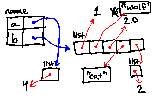
So then when we print a, Python follows its pointer and finds not the original list, but the new single-element list, and so it prints [4]. When we print b, Python follows its pointer and finds our long, modified list (despite the fact that we never explicitly told Python to do anything with b).

A lot of interesting computations on sequences involve processing them one item at a time. Often, they start at the beginning, select each item in turn, do something to it, and continue to the end. This pattern of processing a sequence can be referred to as looping over the sequence. We can write a traversal with a new Python construct: a for loop. To get started, let's consider the following piece of code:

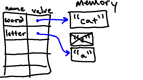
word = "cat"
for letter in word:
    print(letter)
print('done')

In some ways, we can read this like English: for each letter in the string "cat", print that letter (and, after that, print the word "done"). And that's exactly what Python will do. Running this code will produce the following output:

c
a
t
done

From a high-level perspective, we will repeat the code in the indented portion (the body) once for every element in word. Before each repetition, the next character in the string is assigned to the variable letter. Once it has gone through all characters, it will continue on with the rest of the program.

This is a much more complicated structure than some of the others we have looked at, so let's go through this code carefully and keep track of how the environment diagram changes over time.

After we execute the first line (word = "cat"), we have the string "cat" in memory, and it is associated with the name word:

Then we enter the for loop. Before the first line in the body is executed, Python associates the first character from word with the name letter (just the same as if we had done letter = word[0]):

Then we run the loop body for the first time. In doing so, we execute print(letter). Just like it normally would, this involves looking up the value of letter (which, in this case, is "c"), and displaying that value to the screen. So when this line executes, we see a c show up on the screen.

Now, since we've not reached the end of word, we're going to loop again. Before we execute the body again, Python associates the next character from word with the name letter (in this case, just the same as if we had done letter = word[1]):

Then we run the loop body a second time. In doing so, we execute print(letter). Just like before, we looking up the value of letter, but this time we get "a" (since letter was reassigned). So when this line executes this time, we see an a show up on the screen.

Now, since we've still not reached the end of word, we're going to loop again. Again, before we execute the body, Python associates the next character from word with the name letter (in this case, just the same as if we had done letter = word[2]):

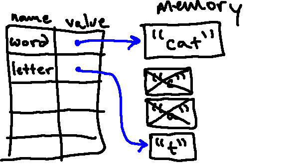
Then we run the loop body once more. In doing so, we again execute print(letter). Just like before, we looking up the value of letter, but this time we get "t" (since letter was once again reassigned). So when this line executes this time, we see a t show up on the screen.

When we are finished looping, our environment diagram still looks like this:

and we return to running the rest of the program. In this case, that just means printing 'done'. But if we had more code, we could reference letter (which is still bound to "t" after exiting the loop).

Note that, as with if statements, the body of a for loop can contain arbitrarily many expressions (and all the indented code will be executed each time through the loop).

Also note that the name letter was an arbitrary choice; we could use any valid variable name there. So we could have made a loop that behaves exactly the same as the one above as follows:

word = "cat"
for arbitrary_variable_name in word:
    print(arbitrary_variable_name)
print('done')

# Note: len(s), where s is a string, produces an int whose value
# is the number of characters in the given string s

count = 0
word = "cow"
print('I am thinking of a nice word.')
print('It has this many letters:')
print(len(word))
print('I will now spell the word for you.')
for i in word:
    print(count)
    print(i)
    count = count + 1
print('The word was:')
print(word)
print('What a nice word.')
print(count)
print(i)

I am thinking of a nice word.
It has this many letters:
3
I will now spell the word for you.
0
c
1
o
2
w
The word was:
cow
What a nice word.
3
w

A common pattern uses append to build up a list of values based on some other list. For example, imagine that we had a list of integers, and we wanted to create a list of the squares of the even numbers in the original list. We could do this with, for example, the following code:

original_list = [7, 4, 8, 2, 9]
new_list = []  # first make an empty list to hold the results
for element in original_list:  # for each number in the original list, do the following:
    if element % 2 == 0:  # if the number is even...
        new_list.append(element ** 2)  # add its square to the new list
print(new_list)

This code will proceed as follows:

• After setting original_list and new_list, Python reaches the for loop.
• The first time through the loop, Python sets element to 7 (the first element in original_list) and runs the loop body.
  • Because 7 % 2 is not equal to 0, Python does not enter the body of the conditional; rather, it moves on.
• Now, Python reassigns element to the next element in the list (4) and enters the loop body.
  • 4 % 2 == 0 evaluates to True, so we enter the body of the conditional, where we add element ** 2 (16) to the end of new_list. If we were to print new_list now, we would see [16].
• Python continues in the same way. It reassigns element to the next element in the list (8) and enters the loop body.
  • 8 % 2 == 0 also evaluates to True, so we enter the body of the conditional again, where we add 64 to the end of new_list. If we were to print new_list now, we would see [16, 64].
• Next, Python reassigns element to 2 (next in the list) and enters the loop body.
  • 2 % 2 == 0 also evaluates to True, so we enter the body of the conditional again, where we add 4 to the end of new_list. If we were to print new_list now, we would see [16, 64, 4].
• Next, Python reassigns element to 9 (next in the list) and enters the loop body again.
  • Because 9 % 2 is not equal to 0, Python does not enter the body of the conditional; rather, it moves on.
• Now that Python has "looped over" every element in original_list, it continues on past the loop to the statement: print(new_list). Printing new_list displays the following to the screen:

  [16, 64, 4]
  

In the sections above, we introduced the notion of looping over a sequence using the for keyword. In a for loop, we performed a computation once for every element in a sequence, setting a particular variable to point to each value in turn.

Sometimes you want to loop over particular values for which constructing a sequence would be a pain. For example, consider printing the squares of all integers from 0 to 24. One way to do this would be to write the following:

for i in [0, 1, 2, 3, 4, 5, 6, 7, 8, 9, 10, 11, 12, 13, 14, 15, 16, 17, 18, 19, 20, 21, 22, 23, 24]:
    print(i**2)

But writing out the list of values we're looping over in this case is a real pain! Conveniently, Python offers us an easier way to build structures of this form, which we can loop over, via range. range can be used to produce a special kind of range object, which, while not exactly the same as a list or tuple, can serve the same purpose when used as part of a for loop.

To do the above more compactly, we could have written:

for i in range(25):
    print(i**2)

If you invoke range with range(4), then it will give you 4 elements, starting from 0 and counting upward. If you invoke it with range(7), it will instead give you seven elements. When used in this way, range will serve the same purpose as a list containing [0, 1, 2, 3] or [0, 1, 2, 3, 4, 5, 6].

Looping over sequence of integers is a fairly common occurrance, and so having range available can really save us a lot of typing (particularly if the sequence of integers you want to loop over is long!).

Much of our discussion above has been about iteration, which is the ability to run a block of statements repeatedly. Earlier, we saw that, using for, we had a way to execute a block of statements once for every element in a sequence. This was very convenient, but sometimes, we do not know a particular sequence of elements over which we want to iterate, nor how many times we would like to run through a loop. Sometimes, we want to repeat a sequence of statements until a particular condition is satisfied.

To this end, Python offers another looping construct, a while loop. A while loop is a lot like a conditional, in that it consists of both a condition and a body and uses the condition to decide whether to execute the body, or to skip it. The difference is: whereas a conditional executed the body exactly once and moved on, a while loop will continue executing the body until the condition no longer evaluates to True. This pattern of flow is represented in this flow chart:

We first enter this diagram from the top. If the condition evaluates to False, then we skip the loop entirely and move on, but if it is True, we enter the body of the loop. The difference from a regular conditional is that if we do execute the body, then once we are done, we jump back and check the condition again (instead of moving on). If the condition is again True, we'll enter the loop again, and so on.

Consider the following example:

n = 5
while n > 0:
    print(n)
    n = n - 1
print('Blastoff!')

You can almost read the while statement as if it were English. It means "While n is greater than 0, display the value of n and then decrement n. When you get to 0, display the word Blastoff!"

Slightly more formally, here is the flow of execution for a while statement:

1. Determine whether the condition is true or false.
2. If false, exit the while statement and continue execution at the next statement.
3. If the condition is true, run the body and then go back to step 1.

As written, the program above will print:

5
4
3
2
1
Blastoff!

It is important, when writing while loops, to make sure that the body of the loop changes the value of one or more variables so that the condition becomes false eventually and the loop terminates. Otherwise the loop will repeat forever, which is called an infinite loop.⁷

In the case of the countdown program, we can prove that the loop terminates: if n is zero or negative, the loop never runs. Otherwise, n gets smaller each time through the loop, so eventually we have to get to 0.

For some other loops, it is not so easy to tell. For example:

n = 27
while n != 1:
    print(n)
    if n % 2 == 0:  # n is even
        n = n / 2
    else:  # n is odd
        n = n*3 + 1

The condition for this loop is n != 1, so the loop will continue until n is 1, which makes the condition false.

Each time through the loop, the program outputs the value of n and then checks whether it is even or odd. If it is even, n is divided by 2. If it is odd, the value of n is replaced with n*3 + 1. For example, if n starts out as 3, the resulting values of n are 3, 10, 5, 16, 8, 4, 2, and 1.

Since n sometimes increases and sometimes decreases, there is no obvious proof that n will ever reach 1, or that the program terminates. For some particular values of n, we can prove termination. For example, if the starting value is a power of two, n will be even every time through the loop until it reaches 1. The previous example ends with such a sequence, starting with 16.

The hard question is whether we can prove that this program terminates for all positive values of n. So far, no one has been able to prove it or disprove it!⁸

6
3.0
10.0
5.0
16.0
8.0
4.0
2.0

Example: Approximating Square Roots

Loops are often used in programs that compute numerical results by starting with an approximate answer and iteratively improving it.

For example, one way of computing square roots is Newton's method. Suppose that you want to know the square root of a. If you start with almost any estimate, x, you can compute a better estimate with the following formula:

For example, if a is 4 and x is 3:

a = 4
x = 3
y = (x + a/x) / 2
print(y)  # prints 2.16666666667

The result is closer to the correct answer (\sqrt{4} = 2). If we repeat the process with the new estimate, it gets even closer:

x = y
y = (x + a/x) / 2
print(y)  # prints 2.00641025641

After a few more updates, the estimate is almost exact:

x = y
y = (x + a/x) / 2
print(y)  # prints 2.00001024003

x = y
y = (x + a/x) / 2
print(y)  # prints 2.00000000003

In general we don't know ahead of time how many steps it takes to get to the right answer, but we know when we get there because the estimate stops changing:

x = y
y = (x + a/x) / 2
print(y)  # prints 2.0
x = y
y = (x + a/x) / 2
print(y)  # prints 2.0

When y == x, we can stop. Here is a loop that starts with an initial estimate, x, and improves it until it stops changing:

a = 4
x = None
y = 2.5
while x != y:
    x = y
    print(x)
    y = (x + a/x) / 2

Note: For most values of a this works fine, but in general it is dangerous to test float equality (for some of the reasons we talked about in the last section, specifically that floats can't accurately represent all numbers!). Rather than checking whether x and y are exactly equal as above, it would be safer to loop until the difference between them of the difference between them becomes small enough (by comparing comparing against some small error margin).

In this reading, we have introduced some new structures, and started moving toward more complicated programs, which can be more difficult to think about. In general, we can attempt to manage this complexity by trying first to break our programs down into small pieces, which can be written and tested independently of the others (this is referred to as modular design because we are thinking of splitting the program into separable modules). It is generally much easier to plan, test, and implement individual pieces as you go, rather than to spend hours writing a big program, and then find it does not work, and have to sift through all your code, trying to find the bugs.

However, even with all the clever design in the world, you will still occasionally find yourself in the (inevitable) position of having a big program with a bug in it; in that case, do not despair! Debugging a program does not require brilliance or creativity or much in the way of insight. What it requires is persistence and a systematic approach, because it requires reasoning not only about what we want, but about how Python will behave in response to our programs (this is why it's so important to have a strong mental model of Python!).

First of all, it is crucial to have a test case (a set of inputs to the program you are trying to debug) and to know what the answer is supposed to be, both for the overall program and for relevant intermediate values. To find a good test case, you might start with some special cases: what if the argument is 0 or the empty list? What if it is negative? Those cases might be easier to sort through first (and are also cases that can be easy to get wrong). Then try more general cases.

For most programs in this class, you should simulate your code by hand using an environment diagram before running it in Python. We know this is tedious, but it really is important for helping you build a strong mental model of how Python behaves. With more experience, you will be able to make these predictions quickly in your head. But for now, draw it out!

Then the question remains: if your program gets your test case(s) wrong, what should you do? Resist the temptation to start changing your program around, just to see if that will fix the problem. Do not change any code until you know what is wrong with what you are doing now, and therefore believe that the change you make is going to correct the problem.

We have a few tools available to us already to this end, which can work reasonably well for small programs: the substitution model for expression evaluation, and environment diagrams. The act of simulating with these tools may help you find your error. It is important to remember that Python doesn't know what you want to do, only what you tell it to do, so you must systematic when going through your code.

Sometimes, you may not be able to find your bug on paper. For those cases, the method we'll advocate centers around debugging systematically using print statements. It is worth noting that nowadays there exist tools other than print to help with debugging (logically called debuggers), but it is very rare even after years of experience programming that we find the need to use such a tool. In our minds, print is still the most straightforward, most powerful, and most general debugging tool in existence.

One good way to use print statements to help in debugging is to use them to display the results of intermediate steps along the way. Depending on the structure of your program, this might be: the values you are looping over (to make sure your bounds are correct), a complete solution to a subproblem, a partial solution to the overall problem. For your chosen location(s), you should print both the quantity of interest and the value you expect that quantity to have. If they are the same, it may be that that part of the code is working properly, and you can try printing in other locations.⁹

One strategy here is to use a variation on binary search. Find a spot roughly halfway through your code at which you can predict the values of variables, or intermediate results your computation. Put a print statement there that lists expected as well as actual values of the variables. Run your test case, and check. If the predicted values match the actual ones, it is likely that the bug occurs after this point in the code; if they do not, then you have a bug prior to this point (of course, you might have a second bug after this point, but you can find that later). Now repeat the process by finding a location halfway between the beginning of the procedure and this point, placing a print statement with expected and actual values, and continuing. In this way you can narrow down the location of the bug. Study that part of the code and see if you can see what is wrong. If not, add some more print statements near the problematic part, and run it again.

The most important rule of debugging is: Don't try to be smart; be systematic and indefatigable! And don't despair!

In this reading, we introduced a few kinds of compound objects (strings, tuples, and lists) and began to expand upon the ideas introduced earlier, by introducing new ways of controlling the order in which Python executes statements (for and while), and using these to give more powerful ways to manipulate compound objects.

In this week's exercises, you'll get some practice with these new pieces, as well as some review on the older pieces. This week we'll really start using Python to solve problems.

In the next set of readings and exercises, we will introduce more tools and a powerful Python built-in type: the dictionary.