 6.s090
Electricity (Part 4: Linear Regression)
Please Log In for full access to the web site.
Note that this link will take you to an external site (https://shimmer.mit.edu) to authenticate, and then you will be redirected back to this page.
In our final installment of the electricity problem, we will find a simple predictive model relating temperature and electricity usage, similar to what you've seen in your statistics and optimization classes.
Before we dive in, let's review various packages in Python that provide regression capabilities.
0.1) Univariate Regression
NumPy performs linear regressions via the numpy.linalg.lstsq function. It uses an iterative method to produce an approximate solution.
For example, if we want to find the best-fit line for the following set of data:
| x_i | y_i |
|---|---|
| 1 | 1 |
| 2 | 2 |
| 3 | 1.3 |
| 4 | 3.75 |
| 5 | 2.25 |
We could use NumPy to formulate this as a least-squares optimization problem:
A = numpy.array([[1, 1],
                 [2, 1],
                 [3, 1],
                 [4, 1],
                 [5, 1]])

b = numpy.array([[1, 2, 1.3, 3.75, 2.25]]).T

print(numpy.linalg.lstsq(A, b))
The first element in the resulting tuple is a NumPy array object representing \left[\begin{array}{c}m\\
b\end{array}\right].
Another package you installed at our kickoff, SciPy, also does linear regressions via its scipy.stats.linregress function. Review the documentation to get a sense for it. As yet another alternative, one can of course manually code up linear regression in Python! We have done so for you in this file, which you may find interesting to examine. You may use all or part of this file in your solution, although you certainly do not need to.
In this exercise, you may use whichever of these alternatives feels most intuitive or familiar to you. Of the three, the manually-coded solution is least efficient, as is to be expected, but not to an extent that will affect this problem.
0.2) Multivariate Linear Regression
The form of the NumPy regression above generalizes to multivariate problems. Consider, for example, the 3-dimensional case, where we have one dependent variable z and two independent variables, x and y. In this case, we have several measured points (x_i, y_i, z_i), and we want to find A, B, and C so as to minimize the sum of squared errors between Ax_i + By_i + C and z_i. If we want to find the best-fit line for the following set of data:
| x_i | y_i | z_i |
|---|---|---|
| 1 | 0 | 1 |
| 2 | 0 | 2 |
| 3 | .7 | 1.3 |
| 4 | .2 | 3.75 |
| 5 | 1 | 2.25 |
We could use NumPy to formulate this as a least-squares optimization problem:
A = numpy.array([[1, 0, 1],
                 [2, 0, 1],
                 [3, 0.7, 1],
                 [4, .2, 1],
                 [5, 1, 1]])

b = numpy.array([[1, 2, 1.3, 3.75, 2.25]]).T

print(numpy.linalg.lstsq(A, b)[0])
SciPy also supports multivariate regressions.
1) Modeling
Now onto finding our predictive model! In order to have a way to test how predictive each of our models is, we will use the first seven years of data to build our model; and we'll use the last three years only as a way to test how predictive our model is. In machine learning, datasets are commonly split into similar "training" and "test" sets.
1.1) Univariate Regression
Let's start by performing a linear regression with average temperature as the independent variable and electricity usage as the dependent variable. Remember only to perform this regression on the first seven years of data. Enter your data to at least 3 decimal places

For the most part, these results match what we would expect. The amount of electricity used increases with the average temperature, and the usage this month predicts for a very cold month (average of 30 degrees) is around the levels we see during the cold winter months in the real data.
Now let's test how predictive our model is. We can do this by calculating Pearson's r between:
- the usages our model predicts for the last three years based on the actual measured temperatures, and
- the actual measured usages during those months
The file linked above has one way to calculate this value; the NumPy and SciPy documentation gives alternatives.
1.2) Analysis
That is a reasonably strong correlation, but we could hope to do better. Let's try to figure out if there is something else going on in the data that we can leverage to do better.
To start, let's generate another plot. This plot should show two pieces of data on the same axes:
- A scatter plot showing electricity usage vs temperature for the first seven years (this is plot #3 from the data visualization exercise), and
- In a different color, the line representing the result from the linear regression.
(Axes: monthly average temperature, usage)
You will want to choose the values over which you plot the line carefully so that you can see both the raw data and the fit.
Upload this graph below:
Do you notice anything interesting about this plot?
It underestimates in hot or cold months, and it overestimates in other months. This might make sense, since ACs are typically run only in the hot summer months and use lots of electricity. In the spring and fall months, people tend not to need either heating or cooling, so their overall usage is lower in those months. In the winter, most homes in Cambridge use natural gas for heating (hence the lower electricity usage), but when it is really cold people sometimes also use electric space heaters (which increases electricity usage).
In the remaining sections, we'll attempt to take more information into account, so that we can make a model that does a better job of predicting electricity usage.
1.3) Other Information
Now let's try to account for the discrepancy above. Here, we'll define three types of days:
- A "hot day" is any day whose low temperature is above 65 degrees
- A "cold day" is any day whose high temperature is less than 40 degrees
- Any other day is a "neutral day"
Augment your CSV from earlier so that it now contains three additional fields. In total, your spreadsheet should now have the following columns:
- Column 1 should contain a year (a number 2007-2016)
- Column 2 should contain a month (a number 1-12)
- Column 3 should contain the electricity usage for that month (in kWh)
- Column 4 should contain the average temperature over that month (in Fahrenheit)
- Column 5 should contain the number of hot days in that month.
- Column 6 should contain the number of cold days in that month.
- Column 7 should contain the number of neutral days in that month.
The first row of the CSV should contain a header ['year', 'month', 'avg_kwh', 'avg_temp', 'num_hot', 'num_cold', 'num_neutral']. The order of the remaining rows should be in chronological order (earliest year / month first, most recent year / month last.)
As an example, the first ten rows of your CSV file should look like the following (but there may be slight differences in calculated avg_temp):
year,month,avg_kwh,avg_temp,num_hot,num_cold,num_neutral
2007,1,554.01,32.74193548387097,0,17,14
2007,2,606.33,26.146428571428572,0,24,4
2007,3,658.42,37.44516129032258,0,11,20
2007,4,526.59,45.166666666666664,0,2,28
2007,5,760.0,61.377419354838715,1,0,30
2007,6,1110.79,68.51666666666667,5,0,25
2007,7,1348.45,72.9,12,0,19
2007,8,1471.95,72.68064516129031,14,0,17
2007,9,1518.79,67.64,3,0,27
Upload your new CSV below:
We will use this CSV moving forward.
1.4) Another Regression
Next, perform another regression on the first seven years' data, this time using all four independent variables (average temperature, hot days, cold days, and neutral days) and a constant term. What are the coefficients associated with each of these variables in the "best fit" line?
1.5) Analysis
Now let's test how predictive this new model is. We can do this by calculating Pearson's r between:
- the usages our model predicts for the last three years based on the actual measured temperatures, and
- the actual measured usages during those months
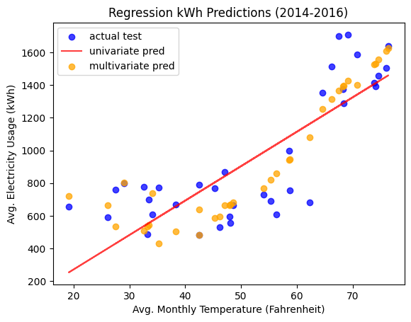
This suggests that our new model (which made use of the extra information) is much more predictive than our original model!
Looking at the plot of the multivariate predictions versus the univariate predications and actual test data below, we can see that the multivariate prediction follows the curve pretty accurately.
Next Exercise: Survey